Lesson 0: Configuring your computer
(c) 2018 Justin Bois. With the exception of pasted graphics, where the source is noted, this work is licensed under a Creative Commons Attribution License CC-BY 4.0. All code contained herein is licensed under an MIT license.
This document was prepared at Caltech with financial support from the Donna and Benjamin M. Rosen Bioengineering Center.

This lesson was generated from an Jupyter notebook. You can download the notebook here.
In this lesson, you will set up a Python computing environment for scientific computing. There are two main ways people set up Python for scientific computing.
- By downloading and installing package by package with tools like apt-get, pip, etc.
- By downloading and installing a Python distribution that contains binaries of many of the scientific packages needed. The major distributions of these are Anaconda and Enthought Canopy. Both contain IDEs.
In this class, we will use Anaconda, with its associated package manager, conda. It has recently become the de facto package manager/distribution for scientific use.
Before we get rolling with the Anaconda distribution, we have some considerations and installations to get out of the way first.
macOS users: Install XCode
If you are using macOS, you should install XCode, if you haven't already. It's a large piece of software, taking up about 5GB on your hard drive, so make sure you have enough space. Please install this ahead of the bootcamp, since if students install this during the bootcamp, it will overwhelm the wireless.
Windows users: Install Git and Chrome or Firefox
We will be using JupyterLab in the bootcamp. It is browser-based, and Chrome, Firefox, and Safari are supported. Internet Explorer is not. Therefore, if you are a Windows user, you need to be sure you have either Chrome of Firefox installed.
Git is installed on Macs with XCode. For Windows users, you need to install Git. You can do this by following the instructions here.
Python 2 vs Python 3
We are at an interesting point in Python's history. Python is currently in version 3.6 (as of June 1, 2017). The problem is that Python 3.x is not backwards compatible with Python 2.x. Many scientific packages were written in Python 2.x and have been very slow to update to Python 3. However, Python 3 is Python's present and future, so all packages eventually need to work in Python 3. Today, most important scientific packages work in Python 3 (and some now only in Python 3). All of the packages we will use do, so we will use Python 3 in this course.
Downloading and installing Anaconda
Downloading and installing Anaconda is simple.
- Go to the Anaconda homepage and download the graphical installer.
- Be sure to download Anaconda for Python 3.6.
- Follow the on-screen instructions for installation. (You may be prompted to install Microsoft Visual Studio Code, which is a good editor, and you may install it if you like, but we will not be using it in the bootcamp.)
That's it! After you do that, you will have a functioning Python distribution.
Launching JupyterLab and a terminal
After installing the Anaconda distribution, you should be able to launch the Anaconda Navigator. If you're using macOS, this is available in your Applications menu. If you are using Windows, you can do this from the Start menu. Launch Anaconda Navigator.
We will be using JupyterLab throughout the bootcamp (more on that in Lesson 1). You should see an option to launch JupyterLab. When you do that, a new browser window or tab will open with JupyterLab running. Within the JupyterLab window, you will have the option to launch a notebook, a console, a terminal, or a text editor. We will use all of these during the bootcamp. For the updating and installation of necessary packages, click on Terminal to launch a terminal. You will get a terminal window (probably black) with a prompt. We refer to this text interface in the terminal as the command line.
The conda package manager
conda is a package manager for keeping all of your packages up-to-date. It has plenty of functionality beyond our basic usage in class, which you can learn more about by reading the docs. We will primarily be using conda to install and update packages.
conda works from the command line. Now that you know how to get a command line prompt, you can start using conda. The first thing we'll do is update conda itself. To do this, enter the following on the command line:
conda update conda
If conda is out of date and needs to be updated, you will be prompted to perform the update. Just type y, and the update will proceed.
Now that conda is updated, we'll use it to see what packages are installed. Type the following on the command line:
conda list
This gives a list of all packages and their versions that are installed. Now, we'll update all packages, so type the following on the command line:
conda update --all
If anything is out of date, you will be prompted to perform the updates. (If everything is up to date, you will just see a list of all the installed packages.) They may even be some downgrades. This happens when there are package conflicts where one package requires an earlier version of another. conda is very smart and figures all of this out for you, so you can almost always say "yes" (or "y") to conda when it prompts you.
Optional installations
We will be using Altair for most of our plotting. By default, Altair only exports graphics as PNG and HTML (which is really all you need, at least for sharing plots and for the paper of the future, which is not a PDF and is interactive). However, many of us are still publishing the paper of the present, which is typically a PDF, and we want vector graphics for our plots. To enable Altair to publish vector graphics, you will need to install the Google Chrome web browser and ChromeDriver. To install Chrome, simply download it and follow the on-screen instructions. You do not need to make it your default browser if you do not want to. To install ChromeDriver, download the most recent ZIPped binary (choose the zip file that matches your operating system). Unzip it, and save the binary to a directory in your PATH. (If you don't know what PATH means, it's ok; we'll cover is in Lesson 2.) If you're using macOS or Linux, you can do the following on the command line, assuming you saved the unzipped file in the Downloads/ folder in your home directory.
mkdir -p /usr/local/bin
mv ~/Downloads/chromedriver /usr/local/bin/
Again, this installation is not necessary for the bootcamp, but will allow you to export SVGs from Altair.
Necessary installations
There are several additional installations you need to do for the bootcamp. First, you need to tell conda in what channels to look for packages. A channel is a URL specifying directories containing conda packages. Not all of the packages are in the default channel of conda, so we will instruct conda to look in the conda-forge and bioconda channels as well as the defaults channel. To do this, execute the following on the command line.
conda config --add channels conda-forge
conda config --add channels bioconda
conda config --add channels defaults
Next, we will install the plotting packages Altair and Holoviews, and Selenium and node.js, which are utilities we won't use directly but may be useful under the hood. To do this, execute the following on the command line.
conda install altair nodejs
Finally, we need to configure JupyterLab to work with Bokeh, which we will use to visualize images.
jupyter labextension install --no-build jupyterlab_bokeh
You may also wish to install a spell-checker (this one isn't necessary). I suspect this spell-checker will either be improved or replaced in the future, but it is all that is currently available (as of June 7, 2018).
jupyter labextension install --no-build @ijmbarr/jupyterlab_spellchecker
After installing all of these extensions, you can rebuild JupyterLab.
jupyter lab build
You should close your JupyterLab session and relaunch it after you have completed the build. As before, after JupyterLab launched, launch a new terminal window so that you can proceed with setting up Git.
Setting up Git
Git features heavily in the bootcamp. We use it for version control and also for sharing files, data, and code we will use in the bootcamp.
Set up a GitHub account
Go to http://github.com/ to get an account. You should register with your Caltech address so you get free private repositories as academics. You should also think carefully about picking your user name. There is a good chance other people in your professional life will see this.
Forking the bootcamp repository
Let's say you want to do some work on a project with code stored in a repository, but you are not an active collaborator. For example, there could be a useful package a lab at another university put on GitHub for a certain kind of image segmentation that is useful for your research. You want to do something almost exactly like the package does, but need to make some small modifications yourself. You want to clone the repository and add a couple functions and maybe modify one or two they already have, leaving much of the rest of the repository untouched. Of course, you also want to update your local copy of all that untouched (but still used) code when the maintainers update it.
This is kind of exactly what you want to do here in the bootcamp. We have a repository that has data sets and a couple tutorials, but you want to write your Python code right in that repository. If I update the data sets, you want to be able to pull in my changes, but still have your code in place.
There is a nice way to do this called forking. To fork a repository on GitHub, simply navigate got the website of the repository and click the Fork button. Be sure you are logged in as yourself when you do this. Here is the GitHub page for the bootcamp.
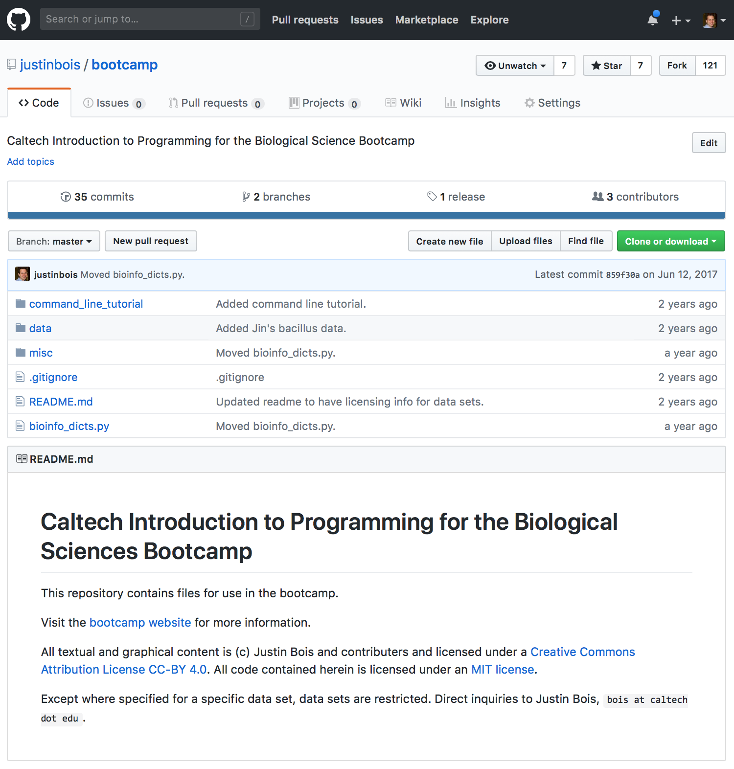
The fork button is in the upper right. Just click the button, and you now have a fork of the bootcamp repository on your GitHub account.
Cloning your fork to your local machine
Now you can clone your fork of the repository to your local machine. We will keep all of your material under version control in a directory called git in your home directory. Do the following on the command line.
mkdir -p ~/git
Now, being sure you are in the ~/git directory, you can clone your forked copy of the repository (not the original bootcamp repository). To do this, navigate your browser to the forked copy of the bootcamp repository on your account (this is where clicking the "Fork" button took you in your browser).
Click the green Clone or download button and copy the URL of the forked repository. Now, you can clone it by doing the following on the command line, making the obvious substitution for the_url_you_just_copied.
cd ~/git
git clone --depth 5 --no-single-branch the_url_you_just_copied
You now have a local copy of your own fork of the bootcamp repository. You can add files and edit it. When you commit and push, it will all be on your account, and the master repository will not see the changes.
Syncing your forked repository to the upstream repository
As I mentioned before, you want to be able to sync your repository with the original bootcamp repository so you can retrieve any updates in it. The original repository is typically called the upstream repository, since presumably you are changing it, so you are downstream. You want the upstream repository to be a remote repository, which is just what we call a repository we track and fetch and merge from. To see which repositories are remote, do the following on the command line.
cd bootcamp
git remote -v
The -v just means "verbose," so it will also tell you the URLs. Entering that now will show a single repository, origin, which you can fetch from and push to. In your case, origin your fork of the bootcamp repository.
We now want to add the upstream repository. To do this, add the original bootcamp repository as the upstream repository.
git remote add upstream https://github.com/justinbois/bootcamp.git
Now try doing git remote -v, and you will see that you are now also tracking the upstream repository.
Checking your distribution
We'll now run a quick test to make sure things are working properly. We will make a quick plot that requires some of the scientific libraries we will use in the bootcamp.
Use the JupyterLab launcher (you can get a new launcher by clicking on the + icon on the left pane of your JupyterLab window) to launch a notebook. In the first cell (the box next to the In [ ]: prompt), paste the code below. To run the code, press Shift+Enter while the cursor is active inside the cell. You should see a plot that looks like the one below. If you do, you have a functioning Python environment for scientific computing!
import numpy as np
import pandas as pd
import altair as alt

# Generate plotting values
t = np.linspace(0, 2*np.pi, 200)
x = 16 * np.sin(t)**3
y = 13 * np.cos(t) - 5 * np.cos(2*t) - 2 * np.cos(3*t) - np.cos(4*t)

# Build a data frame for plotting
df = pd.DataFrame({'x': x,
                   'y': y,
                   't': t})

df_text = pd.DataFrame({'x': [0],
                        'y': [0]})

# Make a plot
heart = alt.Chart(df
        ).mark_line(
            color='red'
        ).encode(
            x='x:Q',
            y='y:Q',
            order='t')

text = alt.Chart(df_text
        ).mark_text(
            text='bootcamp',
            align='center',
            baseline='bottom',
            size=30
        ).encode(
            x='x:Q',
            y='y:Q')

(heart + text).interactive()
