Lesson 13: Introduction to Pandas

---

import numpy as np

# Pandas, conventionally imported as pd
import pandas as pd

---

Throughout your research career, you will undoubtedly need to handle data, possibly lots of data. The data comes in lots of formats, and you will spend much of your time wrangling the data to get it into a usable form.

Pandas is the primary tool in the Python ecosystem for handling data. Its primary object, the DataFrame is extremely useful in wrangling data. We will explore some of that functionality here, and will put it to use in the next lesson.

The data set

We will explore using Pandas with a real data set. We will use a data set published in Beattie, et al., Perceptual impairment in face identification with poor sleep, Royal Society Open Science, 3, 160321, 2016. In this paper, researchers used the Glasgow Facial Matching Test (GMFT) to investigate how sleep deprivation affects a subject’s ability to match faces, as well as the confidence the subject has in those matches. Briefly, the test works by having subjects look at a pair of faces. Two such pairs are shown below.

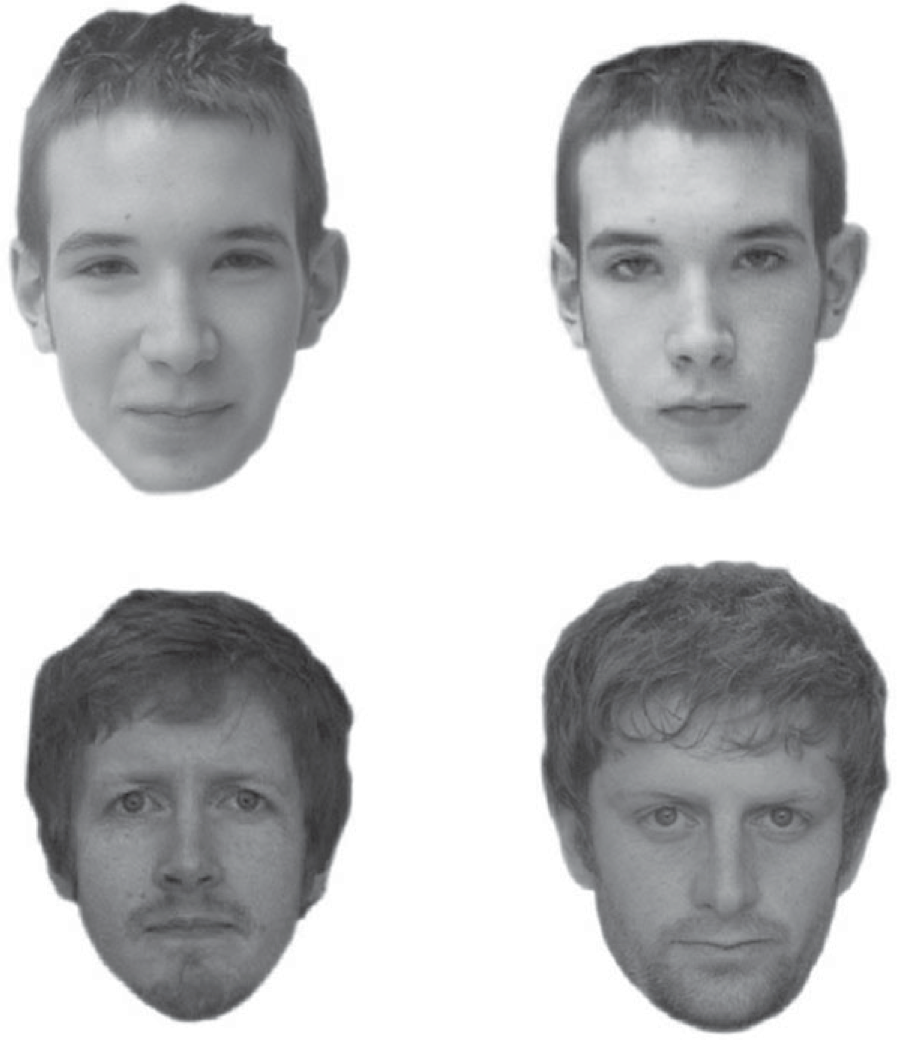
The top two pictures are the same person, the bottom two pictures are different people. For each pair of faces, the subject gets as much time as he or she needs and then says whether or not they are the same person. The subject then rates his or her confidence in the choice.

In this study, subjects also took surveys to determine properties about their sleep. The Sleep Condition Indicator (SCI) is a measure of insomnia disorder over the past month (scores of 16 and below indicate insomnia). The Pittsburgh Sleep Quality Index (PSQI) quantifies how well a subject sleeps in terms of interruptions, latency, etc. A higher score indicates poorer sleep. The Epworth Sleepiness Scale (ESS) assesses daytime drowsiness.

The data set is stored in the file ~/git/bootcamp/data/gfmt_sleep.csv. The contents of this file were adapted from the Excel file posted on the public Dryad repository. (Note this: if you want other people to use and explore your data, make it publicly available.)

This is a CSV file, where CSV stands for comma-separated value. This is a text file that is easily read into data structures in many programming languages. You should generally always store your data in such a format, not necessarily CSV, but a format that is open, has a well-defined specification, and is readable in many contexts. Excel files do not meet these criteria. Neither to .mat files.

Let’s take a look at the CSV file.

!head data/gfmt_sleep.csv

participant number,gender,age,correct hit percentage,correct reject percentage,percent correct,confidence when correct hit,confidence when incorrect hit,confidence when correct reject,confidence when incorrect reject,confidence when correct,confidence when incorrect,sci,psqi,ess
8,f,39,65,80,72.5,91,90,93,83.5,93,90,9,13,2
16,m,42,90,90,90,75.5,55.5,70.5,50,75,50,4,11,7
18,f,31,90,95,92.5,89.5,90,86,81,89,88,10,9,3
22,f,35,100,75,87.5,89.5,*,71,80,88,80,13,8,20
27,f,74,60,65,62.5,68.5,49,61,49,65,49,13,9,12
28,f,61,80,20,50,71,63,31,72.5,64.5,70.5,15,14,2
30,m,32,90,75,82.5,67,56.5,66,65,66,64,16,9,3
33,m,62,45,90,67.5,54,37,65,81.5,62,61,14,9,9
34,f,33,80,100,90,70.5,76.5,64.5,*,68,76.5,14,12,10

The first line contains the headers for each column. They are participant number, gender, age, etc. The data follow. There are two important things to note here. First, notice that the gender column has string data (m or f), while the rest of the data are numeric. Note also that there are some missing data, denoted by the *s in the file.

Given the file I/O skills you recently learned, you could write some functions to parse this file and extract the data you want. You can imagine that this might be kind of painful. However, if the file format is nice and clean, like we more or less have here, we can use pre-built tools. Pandas has a very powerful function, pd.read_csv() that can read in a CSV file and store the contents in a convenient data structure called a data frame. In Pandas, the data type for a data frame is DataFrame, and we will use “data frame” and “DataFrame” interchangeably.

Reading in data

Let’s first look at the doc string of pd.read_csv().

pd.read_csv?

Signature:
pd.read_csv(
    filepath_or_buffer,
    sep=',',
    delimiter=None,
    header='infer',
    names=None,
    index_col=None,
    usecols=None,
    squeeze=False,
    prefix=None,
    mangle_dupe_cols=True,
    dtype=None,
    engine=None,
    converters=None,
    true_values=None,
    false_values=None,
    skipinitialspace=False,
    skiprows=None,
    skipfooter=0,
    nrows=None,
    na_values=None,
    keep_default_na=True,
    na_filter=True,
    verbose=False,
    skip_blank_lines=True,
    parse_dates=False,
    infer_datetime_format=False,
    keep_date_col=False,
    date_parser=None,
    dayfirst=False,
    iterator=False,
    chunksize=None,
    compression='infer',
    thousands=None,
    decimal=b'.',
    lineterminator=None,
    quotechar='"',
    quoting=0,
    doublequote=True,
    escapechar=None,
    comment=None,
    encoding=None,
    dialect=None,
    tupleize_cols=None,
    error_bad_lines=True,
    warn_bad_lines=True,
    delim_whitespace=False,
    low_memory=True,
    memory_map=False,
    float_precision=None,
)
Docstring:
Read a comma-separated values (csv) file into DataFrame.

Also supports optionally iterating or breaking of the file
into chunks.

Additional help can be found in the online docs for
`IO Tools <http://pandas.pydata.org/pandas-docs/stable/io.html>`_.

Parameters
----------
filepath_or_buffer : str, path object, or file-like object
    Any valid string path is acceptable. The string could be a URL. Valid
    URL schemes include http, ftp, s3, and file. For file URLs, a host is
    expected. A local file could be: file://localhost/path/to/table.csv.

    If you want to pass in a path object, pandas accepts either
    ``pathlib.Path`` or ``py._path.local.LocalPath``.

    By file-like object, we refer to objects with a ``read()`` method, such as
    a file handler (e.g. via builtin ``open`` function) or ``StringIO``.
sep : str, default ','
    Delimiter to use. If sep is None, the C engine cannot automatically detect
    the separator, but the Python parsing engine can, meaning the latter will
    be used and automatically detect the separator by Python's builtin sniffer
    tool, ``csv.Sniffer``. In addition, separators longer than 1 character and
    different from ``'\s+'`` will be interpreted as regular expressions and
    will also force the use of the Python parsing engine. Note that regex
    delimiters are prone to ignoring quoted data. Regex example: ``'\r\t'``.
delimiter : str, default ``None``
    Alias for sep.
header : int, list of int, default 'infer'
    Row number(s) to use as the column names, and the start of the
    data.  Default behavior is to infer the column names: if no names
    are passed the behavior is identical to ``header=0`` and column
    names are inferred from the first line of the file, if column
    names are passed explicitly then the behavior is identical to
    ``header=None``. Explicitly pass ``header=0`` to be able to
    replace existing names. The header can be a list of integers that
    specify row locations for a multi-index on the columns
    e.g. [0,1,3]. Intervening rows that are not specified will be
    skipped (e.g. 2 in this example is skipped). Note that this
    parameter ignores commented lines and empty lines if
    ``skip_blank_lines=True``, so ``header=0`` denotes the first line of
    data rather than the first line of the file.
names : array-like, optional
    List of column names to use. If file contains no header row, then you
    should explicitly pass ``header=None``. Duplicates in this list will cause
    a ``UserWarning`` to be issued.
index_col : int, sequence or bool, optional
    Column to use as the row labels of the DataFrame. If a sequence is given, a
    MultiIndex is used. If you have a malformed file with delimiters at the end
    of each line, you might consider ``index_col=False`` to force pandas to
    not use the first column as the index (row names).
usecols : list-like or callable, optional
    Return a subset of the columns. If list-like, all elements must either
    be positional (i.e. integer indices into the document columns) or strings
    that correspond to column names provided either by the user in `names` or
    inferred from the document header row(s). For example, a valid list-like
    `usecols` parameter would be ``[0, 1, 2]`` or ``['foo', 'bar', 'baz']``.
    Element order is ignored, so ``usecols=[0, 1]`` is the same as ``[1, 0]``.
    To instantiate a DataFrame from ``data`` with element order preserved use
    ``pd.read_csv(data, usecols=['foo', 'bar'])[['foo', 'bar']]`` for columns
    in ``['foo', 'bar']`` order or
    ``pd.read_csv(data, usecols=['foo', 'bar'])[['bar', 'foo']]``
    for ``['bar', 'foo']`` order.

    If callable, the callable function will be evaluated against the column
    names, returning names where the callable function evaluates to True. An
    example of a valid callable argument would be ``lambda x: x.upper() in
    ['AAA', 'BBB', 'DDD']``. Using this parameter results in much faster
    parsing time and lower memory usage.
squeeze : bool, default False
    If the parsed data only contains one column then return a Series.
prefix : str, optional
    Prefix to add to column numbers when no header, e.g. 'X' for X0, X1, ...
mangle_dupe_cols : bool, default True
    Duplicate columns will be specified as 'X', 'X.1', ...'X.N', rather than
    'X'...'X'. Passing in False will cause data to be overwritten if there
    are duplicate names in the columns.
dtype : Type name or dict of column -> type, optional
    Data type for data or columns. E.g. {'a': np.float64, 'b': np.int32,
    'c': 'Int64'}
    Use `str` or `object` together with suitable `na_values` settings
    to preserve and not interpret dtype.
    If converters are specified, they will be applied INSTEAD
    of dtype conversion.
engine : {'c', 'python'}, optional
    Parser engine to use. The C engine is faster while the python engine is
    currently more feature-complete.
converters : dict, optional
    Dict of functions for converting values in certain columns. Keys can either
    be integers or column labels.
true_values : list, optional
    Values to consider as True.
false_values : list, optional
    Values to consider as False.
skipinitialspace : bool, default False
    Skip spaces after delimiter.
skiprows : list-like, int or callable, optional
    Line numbers to skip (0-indexed) or number of lines to skip (int)
    at the start of the file.

    If callable, the callable function will be evaluated against the row
    indices, returning True if the row should be skipped and False otherwise.
    An example of a valid callable argument would be ``lambda x: x in [0, 2]``.
skipfooter : int, default 0
    Number of lines at bottom of file to skip (Unsupported with engine='c').
nrows : int, optional
    Number of rows of file to read. Useful for reading pieces of large files.
na_values : scalar, str, list-like, or dict, optional
    Additional strings to recognize as NA/NaN. If dict passed, specific
    per-column NA values.  By default the following values are interpreted as
    NaN: '', '#N/A', '#N/A N/A', '#NA', '-1.#IND', '-1.#QNAN', '-NaN', '-nan',
    '1.#IND', '1.#QNAN', 'N/A', 'NA', 'NULL', 'NaN', 'n/a', 'nan',
    'null'.
keep_default_na : bool, default True
    Whether or not to include the default NaN values when parsing the data.
    Depending on whether `na_values` is passed in, the behavior is as follows:

    * If `keep_default_na` is True, and `na_values` are specified, `na_values`
      is appended to the default NaN values used for parsing.
    * If `keep_default_na` is True, and `na_values` are not specified, only
      the default NaN values are used for parsing.
    * If `keep_default_na` is False, and `na_values` are specified, only
      the NaN values specified `na_values` are used for parsing.
    * If `keep_default_na` is False, and `na_values` are not specified, no
      strings will be parsed as NaN.

    Note that if `na_filter` is passed in as False, the `keep_default_na` and
    `na_values` parameters will be ignored.
na_filter : bool, default True
    Detect missing value markers (empty strings and the value of na_values). In
    data without any NAs, passing na_filter=False can improve the performance
    of reading a large file.
verbose : bool, default False
    Indicate number of NA values placed in non-numeric columns.
skip_blank_lines : bool, default True
    If True, skip over blank lines rather than interpreting as NaN values.
parse_dates : bool or list of int or names or list of lists or dict, default False
    The behavior is as follows:

    * boolean. If True -> try parsing the index.
    * list of int or names. e.g. If [1, 2, 3] -> try parsing columns 1, 2, 3
      each as a separate date column.
    * list of lists. e.g.  If [[1, 3]] -> combine columns 1 and 3 and parse as
      a single date column.
    * dict, e.g. {'foo' : [1, 3]} -> parse columns 1, 3 as date and call
      result 'foo'

    If a column or index cannot be represented as an array of datetimes,
    say because of an unparseable value or a mixture of timezones, the column
    or index will be returned unaltered as an object data type. For
    non-standard datetime parsing, use ``pd.to_datetime`` after
    ``pd.read_csv``. To parse an index or column with a mixture of timezones,
    specify ``date_parser`` to be a partially-applied
    :func:`pandas.to_datetime` with ``utc=True``. See
    :ref:`io.csv.mixed_timezones` for more.

    Note: A fast-path exists for iso8601-formatted dates.
infer_datetime_format : bool, default False
    If True and `parse_dates` is enabled, pandas will attempt to infer the
    format of the datetime strings in the columns, and if it can be inferred,
    switch to a faster method of parsing them. In some cases this can increase
    the parsing speed by 5-10x.
keep_date_col : bool, default False
    If True and `parse_dates` specifies combining multiple columns then
    keep the original columns.
date_parser : function, optional
    Function to use for converting a sequence of string columns to an array of
    datetime instances. The default uses ``dateutil.parser.parser`` to do the
    conversion. Pandas will try to call `date_parser` in three different ways,
    advancing to the next if an exception occurs: 1) Pass one or more arrays
    (as defined by `parse_dates`) as arguments; 2) concatenate (row-wise) the
    string values from the columns defined by `parse_dates` into a single array
    and pass that; and 3) call `date_parser` once for each row using one or
    more strings (corresponding to the columns defined by `parse_dates`) as
    arguments.
dayfirst : bool, default False
    DD/MM format dates, international and European format.
iterator : bool, default False
    Return TextFileReader object for iteration or getting chunks with
    ``get_chunk()``.
chunksize : int, optional
    Return TextFileReader object for iteration.
    See the `IO Tools docs
    <http://pandas.pydata.org/pandas-docs/stable/io.html#io-chunking>`_
    for more information on ``iterator`` and ``chunksize``.
compression : {'infer', 'gzip', 'bz2', 'zip', 'xz', None}, default 'infer'
    For on-the-fly decompression of on-disk data. If 'infer' and
    `filepath_or_buffer` is path-like, then detect compression from the
    following extensions: '.gz', '.bz2', '.zip', or '.xz' (otherwise no
    decompression). If using 'zip', the ZIP file must contain only one data
    file to be read in. Set to None for no decompression.

    .. versionadded:: 0.18.1 support for 'zip' and 'xz' compression.

thousands : str, optional
    Thousands separator.
decimal : str, default '.'
    Character to recognize as decimal point (e.g. use ',' for European data).
lineterminator : str (length 1), optional
    Character to break file into lines. Only valid with C parser.
quotechar : str (length 1), optional
    The character used to denote the start and end of a quoted item. Quoted
    items can include the delimiter and it will be ignored.
quoting : int or csv.QUOTE_* instance, default 0
    Control field quoting behavior per ``csv.QUOTE_*`` constants. Use one of
    QUOTE_MINIMAL (0), QUOTE_ALL (1), QUOTE_NONNUMERIC (2) or QUOTE_NONE (3).
doublequote : bool, default ``True``
   When quotechar is specified and quoting is not ``QUOTE_NONE``, indicate
   whether or not to interpret two consecutive quotechar elements INSIDE a
   field as a single ``quotechar`` element.
escapechar : str (length 1), optional
    One-character string used to escape other characters.
comment : str, optional
    Indicates remainder of line should not be parsed. If found at the beginning
    of a line, the line will be ignored altogether. This parameter must be a
    single character. Like empty lines (as long as ``skip_blank_lines=True``),
    fully commented lines are ignored by the parameter `header` but not by
    `skiprows`. For example, if ``comment='#'``, parsing
    ``#empty\na,b,c\n1,2,3`` with ``header=0`` will result in 'a,b,c' being
    treated as the header.
encoding : str, optional
    Encoding to use for UTF when reading/writing (ex. 'utf-8'). `List of Python
    standard encodings
    <https://docs.python.org/3/library/codecs.html#standard-encodings>`_ .
dialect : str or csv.Dialect, optional
    If provided, this parameter will override values (default or not) for the
    following parameters: `delimiter`, `doublequote`, `escapechar`,
    `skipinitialspace`, `quotechar`, and `quoting`. If it is necessary to
    override values, a ParserWarning will be issued. See csv.Dialect
    documentation for more details.
tupleize_cols : bool, default False
    Leave a list of tuples on columns as is (default is to convert to
    a MultiIndex on the columns).

    .. deprecated:: 0.21.0
       This argument will be removed and will always convert to MultiIndex

error_bad_lines : bool, default True
    Lines with too many fields (e.g. a csv line with too many commas) will by
    default cause an exception to be raised, and no DataFrame will be returned.
    If False, then these "bad lines" will dropped from the DataFrame that is
    returned.
warn_bad_lines : bool, default True
    If error_bad_lines is False, and warn_bad_lines is True, a warning for each
    "bad line" will be output.
delim_whitespace : bool, default False
    Specifies whether or not whitespace (e.g. ``' '`` or ``'    '``) will be
    used as the sep. Equivalent to setting ``sep='\s+'``. If this option
    is set to True, nothing should be passed in for the ``delimiter``
    parameter.

    .. versionadded:: 0.18.1 support for the Python parser.

low_memory : bool, default True
    Internally process the file in chunks, resulting in lower memory use
    while parsing, but possibly mixed type inference.  To ensure no mixed
    types either set False, or specify the type with the `dtype` parameter.
    Note that the entire file is read into a single DataFrame regardless,
    use the `chunksize` or `iterator` parameter to return the data in chunks.
    (Only valid with C parser).
memory_map : bool, default False
    If a filepath is provided for `filepath_or_buffer`, map the file object
    directly onto memory and access the data directly from there. Using this
    option can improve performance because there is no longer any I/O overhead.
float_precision : str, optional
    Specifies which converter the C engine should use for floating-point
    values. The options are `None` for the ordinary converter,
    `high` for the high-precision converter, and `round_trip` for the
    round-trip converter.

Returns
-------
DataFrame or TextParser
    A comma-separated values (csv) file is returned as two-dimensional
    data structure with labeled axes.

See Also
--------
to_csv : Write DataFrame to a comma-separated values (csv) file.
read_csv : Read a comma-separated values (csv) file into DataFrame.
read_fwf : Read a table of fixed-width formatted lines into DataFrame.

Examples
--------
>>> pd.read_csv('data.csv')  # doctest: +SKIP
File:      ~/opt/anaconda3/lib/python3.7/site-packages/pandas/io/parsers.py
Type:      function

Holy cow! There are so many options we can specify for reading in a CSV file. You will likely find reasons to use many of these throughout your research. For this particular data set, we really only need the na_values kwarg. This specifies what characters signify that a data point is missing. The resulting data frame is populated with a NaN, or not-a-number, wherever this character is present in the file. In this case, we want na_values='*'. So, let’s load in the data set.

df = pd.read_csv('data/gfmt_sleep.csv', na_values='*')

# Check the type
type(df)

pandas.core.frame.DataFrame

We now have the data stored in a data frame. We can look at it in the Jupyter notebook, since Jupyter will display it in a well-organized, pretty way.

df

	participant number	gender	age	correct hit percentage	correct reject percentage	percent correct	confidence when correct hit	confidence when incorrect hit	confidence when correct reject	confidence when incorrect reject	confidence when correct	confidence when incorrect	sci	psqi	ess
0	8	f	39	65	80	72.5	91.0	90.0	93.0	83.5	93.0	90.0	9	13	2
1	16	m	42	90	90	90.0	75.5	55.5	70.5	50.0	75.0	50.0	4	11	7
2	18	f	31	90	95	92.5	89.5	90.0	86.0	81.0	89.0	88.0	10	9	3
3	22	f	35	100	75	87.5	89.5	NaN	71.0	80.0	88.0	80.0	13	8	20
4	27	f	74	60	65	62.5	68.5	49.0	61.0	49.0	65.0	49.0	13	9	12
5	28	f	61	80	20	50.0	71.0	63.0	31.0	72.5	64.5	70.5	15	14	2
6	30	m	32	90	75	82.5	67.0	56.5	66.0	65.0	66.0	64.0	16	9	3
7	33	m	62	45	90	67.5	54.0	37.0	65.0	81.5	62.0	61.0	14	9	9
8	34	f	33	80	100	90.0	70.5	76.5	64.5	NaN	68.0	76.5	14	12	10
9	35	f	53	100	50	75.0	74.5	NaN	60.5	65.0	71.0	65.0	14	8	7
10	38	f	41	70	55	62.5	82.0	61.5	73.0	69.0	82.0	64.0	14	5	19
11	41	f	36	90	100	95.0	76.5	75.5	75.0	NaN	76.0	75.5	15	7	0
12	46	f	40	95	65	80.0	80.0	89.0	79.0	58.5	79.5	63.0	10	12	8
13	49	f	24	85	75	80.0	58.0	50.0	49.0	68.0	55.0	59.0	14	13	4
14	55	f	32	75	55	65.0	85.0	81.0	85.0	86.0	85.0	83.5	5	13	7
15	71	f	40	40	100	70.0	69.0	56.0	70.0	NaN	70.0	56.0	0	11	14
16	76	f	61	100	40	70.0	69.5	NaN	44.5	73.0	54.5	73.0	16	4	12
17	77	f	42	70	90	80.0	87.0	72.0	90.5	43.5	88.5	64.0	11	10	10
18	78	m	31	100	70	85.0	92.0	NaN	81.0	60.0	87.5	60.0	14	6	11
19	80	m	28	100	50	75.0	100.0	NaN	100.0	100.0	100.0	100.0	12	7	12
20	89	f	26	60	80	70.0	70.0	77.0	82.0	67.5	77.0	70.5	14	8	1
21	90	m	45	100	95	97.5	100.0	NaN	100.0	100.0	100.0	100.0	14	9	6
22	93	f	28	100	75	87.5	89.5	NaN	67.0	60.0	80.0	60.0	16	7	4
23	100	f	44	65	25	45.0	62.0	72.0	87.0	77.0	69.5	73.5	1	15	6
24	101	f	28	100	40	70.0	87.0	NaN	68.0	54.0	81.0	54.0	14	7	2
25	1	f	42	80	65	72.5	51.5	44.5	43.0	49.0	51.0	49.0	29	1	5
26	2	f	45	80	90	85.0	75.0	55.5	80.0	75.0	78.5	67.0	19	5	1
27	3	f	16	70	80	75.0	70.0	57.0	54.0	53.0	57.0	54.5	23	1	3
28	4	f	21	70	65	67.5	63.5	64.0	50.0	50.0	60.0	50.0	26	5	4
29	5	f	18	90	100	95.0	76.5	83.0	80.0	NaN	80.0	83.0	21	7	5
...	...	...	...	...	...	...	...	...	...	...	...	...	...	...	...
72	64	f	69	95	80	87.5	80.0	65.0	78.5	70.5	80.0	70.0	31	1	1
73	65	f	31	100	95	97.5	98.0	NaN	90.0	40.0	92.0	40.0	27	4	4
74	66	f	44	90	95	92.5	87.0	47.5	69.0	87.0	83.0	67.0	32	1	2
75	67	f	25	100	100	100.0	61.5	NaN	58.5	NaN	60.5	NaN	28	8	9
76	68	f	45	70	50	60.0	80.5	51.5	63.0	69.0	72.5	61.5	25	4	1
77	69	f	47	90	100	95.0	100.0	NaN	71.5	83.0	97.5	83.0	30	2	2
78	70	f	33	85	70	77.5	70.0	38.0	58.5	65.0	68.0	40.0	21	7	12
79	72	f	18	80	75	77.5	67.5	51.5	66.0	57.0	67.0	53.0	29	4	6
80	73	f	74	85	80	82.5	66.0	55.0	63.0	50.5	65.0	55.0	20	1	5
81	74	m	21	40	40	40.0	90.5	80.0	74.5	83.0	82.0	81.0	22	7	5
82	75	f	45	80	95	87.5	74.0	67.0	76.0	17.0	75.0	64.0	23	4	4
83	79	f	37	90	80	85.0	95.5	68.0	83.5	83.0	94.0	71.0	20	5	9
84	81	m	41	90	85	87.5	80.0	59.5	70.0	41.0	77.0	59.0	17	6	3
85	82	f	41	80	75	77.5	94.5	61.5	86.0	74.0	92.0	67.0	27	4	8
86	83	f	34	90	35	62.5	81.0	52.0	71.0	58.0	81.0	58.0	27	2	6
87	84	f	39	75	70	72.5	57.0	57.0	59.5	50.0	58.0	50.0	22	3	10
88	85	f	18	85	85	85.0	93.0	92.0	91.0	89.0	91.5	91.0	25	4	21
89	86	f	31	100	85	92.5	100.0	NaN	100.0	50.0	100.0	50.0	30	3	5
90	87	m	26	95	75	85.0	85.0	88.0	82.0	82.0	85.0	85.0	32	1	5
91	88	m	66	60	85	72.5	67.5	66.0	74.0	57.0	74.0	64.0	30	5	9
92	91	m	62	100	80	90.0	81.0	NaN	74.5	82.0	79.5	82.0	32	2	1
93	92	m	22	85	95	90.0	66.0	56.0	72.0	63.0	70.5	59.5	28	1	8
94	94	f	41	35	75	55.0	55.0	61.0	80.0	57.0	72.0	60.0	31	1	11
95	95	m	46	95	80	87.5	90.0	75.0	80.0	80.0	85.0	75.0	29	3	5
96	96	f	56	70	50	60.0	63.0	52.5	67.5	65.5	64.0	59.5	26	6	7
97	97	f	23	70	85	77.5	77.0	66.5	77.0	77.5	77.0	74.0	20	8	10
98	98	f	70	90	85	87.5	65.5	85.5	87.0	80.0	74.0	80.0	19	8	7
99	99	f	24	70	80	75.0	61.5	81.0	70.0	61.0	65.0	81.0	31	2	15
100	102	f	40	75	65	70.0	53.0	37.0	84.0	52.0	81.0	51.0	22	4	7
101	103	f	33	85	40	62.5	80.0	27.0	31.0	82.5	81.0	73.0	24	5	7

102 rows × 15 columns

This is a nice representation of the data, but we really do not need to display that much. Instead, we can use the head() method of data frames to look at the first few rows.

df.head()

	participant number	gender	age	correct hit percentage	correct reject percentage	percent correct	confidence when correct hit	confidence when incorrect hit	confidence when correct reject	confidence when incorrect reject	confidence when correct	confidence when incorrect	sci	psqi	ess
0	8	f	39	65	80	72.5	91.0	90.0	93.0	83.5	93.0	90.0	9	13	2
1	16	m	42	90	90	90.0	75.5	55.5	70.5	50.0	75.0	50.0	4	11	7
2	18	f	31	90	95	92.5	89.5	90.0	86.0	81.0	89.0	88.0	10	9	3
3	22	f	35	100	75	87.5	89.5	NaN	71.0	80.0	88.0	80.0	13	8	20
4	27	f	74	60	65	62.5	68.5	49.0	61.0	49.0	65.0	49.0	13	9	12

This is more manageable and gives us an overview of what the columns are. Note also the the missing data was populated with NaN.

Indexing data frames

The data frame is a convenient data structure for many reasons that will become clear as we start exploring. Let’s start by looking at how data frames are indexed. Let’s try to look at the first row.

df[0]

---------------------------------------------------------------------------
KeyError                                  Traceback (most recent call last)
~/opt/anaconda3/lib/python3.7/site-packages/pandas/core/indexes/base.py in get_loc(self, key, method, tolerance)
   2656             try:
-> 2657                 return self._engine.get_loc(key)
   2658             except KeyError:

pandas/_libs/index.pyx in pandas._libs.index.IndexEngine.get_loc()

pandas/_libs/index.pyx in pandas._libs.index.IndexEngine.get_loc()

pandas/_libs/hashtable_class_helper.pxi in pandas._libs.hashtable.PyObjectHashTable.get_item()

pandas/_libs/hashtable_class_helper.pxi in pandas._libs.hashtable.PyObjectHashTable.get_item()

KeyError: 0

During handling of the above exception, another exception occurred:

KeyError                                  Traceback (most recent call last)
<ipython-input-7-ad11118bc8f3> in <module>
----> 1 df[0]

~/opt/anaconda3/lib/python3.7/site-packages/pandas/core/frame.py in __getitem__(self, key)
   2925             if self.columns.nlevels > 1:
   2926                 return self._getitem_multilevel(key)
-> 2927             indexer = self.columns.get_loc(key)
   2928             if is_integer(indexer):
   2929                 indexer = [indexer]

~/opt/anaconda3/lib/python3.7/site-packages/pandas/core/indexes/base.py in get_loc(self, key, method, tolerance)
   2657                 return self._engine.get_loc(key)
   2658             except KeyError:
-> 2659                 return self._engine.get_loc(self._maybe_cast_indexer(key))
   2660         indexer = self.get_indexer([key], method=method, tolerance=tolerance)
   2661         if indexer.ndim > 1 or indexer.size > 1:

pandas/_libs/index.pyx in pandas._libs.index.IndexEngine.get_loc()

pandas/_libs/index.pyx in pandas._libs.index.IndexEngine.get_loc()

pandas/_libs/hashtable_class_helper.pxi in pandas._libs.hashtable.PyObjectHashTable.get_item()

pandas/_libs/hashtable_class_helper.pxi in pandas._libs.hashtable.PyObjectHashTable.get_item()

KeyError: 0

Yikes! Lots of errors. The problem is that we tried to index numerically by row. We index DataFrames, by columns. And there is no column that has the name 0 in this data frame, though there could be. Instead, a might want to look at the column with the percentage of correct face matching tasks.

df['percent correct']

0       72.5
1       90.0
2       92.5
3       87.5
4       62.5
5       50.0
6       82.5
7       67.5
8       90.0
9       75.0
10      62.5
11      95.0
12      80.0
13      80.0
14      65.0
15      70.0
16      70.0
17      80.0
18      85.0
19      75.0
20      70.0
21      97.5
22      87.5
23      45.0
24      70.0
25      72.5
26      85.0
27      75.0
28      67.5
29      95.0
       ...
72      87.5
73      97.5
74      92.5
75     100.0
76      60.0
77      95.0
78      77.5
79      77.5
80      82.5
81      40.0
82      87.5
83      85.0
84      87.5
85      77.5
86      62.5
87      72.5
88      85.0
89      92.5
90      85.0
91      72.5
92      90.0
93      90.0
94      55.0
95      87.5
96      60.0
97      77.5
98      87.5
99      75.0
100     70.0
101     62.5
Name: percent correct, Length: 102, dtype: float64

This gave us the numbers we were after. Notice that when it was printed, the index of the rows came along with it. If we wanted to pull out a single percentage correct, say corresponding to index 4, we can do that.

df['percent correct'][4]

62.5

However, this is not the preferred way to do this. It is better to use .loc. This give the location in the data frame we want.

df.loc[4, 'percent correct']

62.5

It is also important to note that row indices need not be integers. And you should not count on them being integers. In practice you will almost never use row indices, but rather use Boolean indexing.

Boolean indexing of data frames

Let’s say I wanted the percent correct of participant number 42. I can use Boolean indexing to specify the row. Specifically, I want the row for which df['participant number'] == 42. You can essentially plop this syntax directly when using .loc.

df.loc[df['participant number'] == 42, 'percent correct']

54    85.0
Name: percent correct, dtype: float64

If I want to pull the whole record for that participant, I can use : for the column index.

df.loc[df['participant number'] == 42, :]

	participant number	gender	age	correct hit percentage	correct reject percentage	percent correct	confidence when correct hit	confidence when incorrect hit	confidence when correct reject	confidence when incorrect reject	confidence when correct	confidence when incorrect	sci	psqi	ess
54	42	m	29	100	70	85.0	75.0	NaN	64.5	43.0	74.0	43.0	32	1	6

Notice that the index, 54, comes along for the ride, but we do not need it.

Now, let’s pull out all records of females under the age of 21. We can again use Boolean indexing, but we need to use an & operator. We did not cover this bitwise operator before, but the syntax is self-explanatory in the example below. Note that it is important that each Boolean operation you are doing is in parentheses because of the precedence of the operators involved.

df.loc[(df['age'] < 21) & (df['gender'] == 'f'), :]

	participant number	gender	age	correct hit percentage	correct reject percentage	percent correct	confidence when correct hit	confidence when incorrect hit	confidence when correct reject	confidence when incorrect reject	confidence when correct	confidence when incorrect	sci	psqi	ess
27	3	f	16	70	80	75.0	70.0	57.0	54.0	53.0	57.0	54.5	23	1	3
29	5	f	18	90	100	95.0	76.5	83.0	80.0	NaN	80.0	83.0	21	7	5
66	58	f	16	85	85	85.0	55.0	30.0	50.0	40.0	52.5	35.0	29	2	11
79	72	f	18	80	75	77.5	67.5	51.5	66.0	57.0	67.0	53.0	29	4	6
88	85	f	18	85	85	85.0	93.0	92.0	91.0	89.0	91.5	91.0	25	4	21

We can do something even more complicated, like pull out all females under 30 who got more than 85% of the face matching tasks correct. The code is clearer if we set up our Boolean indexing first, as follows.

inds = (df['age'] < 30) & (df['gender'] == 'f') & (df['percent correct'] > 85)

# Take a look
inds

0      False
1      False
2      False
3      False
4      False
5      False
6      False
7      False
8      False
9      False
10     False
11     False
12     False
13     False
14     False
15     False
16     False
17     False
18     False
19     False
20     False
21     False
22      True
23     False
24     False
25     False
26     False
27     False
28     False
29      True
       ...
72     False
73     False
74     False
75      True
76     False
77     False
78     False
79     False
80     False
81     False
82     False
83     False
84     False
85     False
86     False
87     False
88     False
89     False
90     False
91     False
92     False
93     False
94     False
95     False
96     False
97     False
98     False
99     False
100    False
101    False
Length: 102, dtype: bool

Notice that inds is an array (actually a Pandas Series, essentially a DataFrame with one column) of Trues and Falses. When we index with it using .loc, we get back rows where inds is True.

df.loc[inds, :]

	participant number	gender	age	correct hit percentage	correct reject percentage	percent correct	confidence when correct hit	confidence when incorrect hit	confidence when correct reject	confidence when incorrect reject	confidence when correct	confidence when incorrect	sci	psqi	ess
22	93	f	28	100	75	87.5	89.5	NaN	67.0	60.0	80.0	60.0	16	7	4
29	5	f	18	90	100	95.0	76.5	83.0	80.0	NaN	80.0	83.0	21	7	5
30	6	f	28	95	80	87.5	100.0	85.0	94.0	61.0	99.0	65.0	19	7	12
33	10	f	25	100	100	100.0	90.0	NaN	85.0	NaN	90.0	NaN	17	10	11
56	44	f	21	85	90	87.5	66.0	29.0	70.0	29.0	67.0	29.0	26	7	18
58	48	f	23	90	85	87.5	67.0	47.0	69.0	40.0	67.0	40.0	18	6	8
60	51	f	24	85	95	90.0	97.0	41.0	74.0	73.0	83.0	55.5	29	1	7
75	67	f	25	100	100	100.0	61.5	NaN	58.5	NaN	60.5	NaN	28	8	9

Of interest in this exercise in Boolean indexing is that we never had to write a loop. To produce our indices, we could have done the following.

# Initialize array of Boolean indices
inds = [False] * len(df)

# Iterate over the rows of the DataFrame to check if the row should be included
for i, r in df.iterrows():
    if r['age'] < 30 and r['gender'] == 'f' and r['percent correct'] > 85:
        inds[i] = True

# Make our seleciton with Boolean indexing
df.loc[inds, :]

	participant number	gender	age	correct hit percentage	correct reject percentage	percent correct	confidence when correct hit	confidence when incorrect hit	confidence when correct reject	confidence when incorrect reject	confidence when correct	confidence when incorrect	sci	psqi	ess
22	93	f	28	100	75	87.5	89.5	NaN	67.0	60.0	80.0	60.0	16	7	4
29	5	f	18	90	100	95.0	76.5	83.0	80.0	NaN	80.0	83.0	21	7	5
30	6	f	28	95	80	87.5	100.0	85.0	94.0	61.0	99.0	65.0	19	7	12
33	10	f	25	100	100	100.0	90.0	NaN	85.0	NaN	90.0	NaN	17	10	11
56	44	f	21	85	90	87.5	66.0	29.0	70.0	29.0	67.0	29.0	26	7	18
58	48	f	23	90	85	87.5	67.0	47.0	69.0	40.0	67.0	40.0	18	6	8
60	51	f	24	85	95	90.0	97.0	41.0	74.0	73.0	83.0	55.5	29	1	7
75	67	f	25	100	100	100.0	61.5	NaN	58.5	NaN	60.5	NaN	28	8	9

This feature, where the looping is done automatically on Pandas objects like data frames, is very powerful and saves us writing lots of lines of code. This example also showed how to use the iterrows() method of a data frame to iterate over the rows of a data frame. It is actually rare that you will need to do that, as we’ll show next when computing with data frames.

Calculating with data frames

Recall that a subject is said to suffer from insomnia if he or she has an SCI of 16 or below. We might like to add a column to the data frame that specifies whether or not the subject suffers from insomnia. We can conveniently compute with columns. This is done elementwise.

df['sci'] <= 16

0       True
1       True
2       True
3       True
4       True
5       True
6       True
7       True
8       True
9       True
10      True
11      True
12      True
13      True
14      True
15      True
16      True
17      True
18      True
19      True
20      True
21      True
22      True
23      True
24      True
25     False
26     False
27     False
28     False
29     False
       ...
72     False
73     False
74     False
75     False
76     False
77     False
78     False
79     False
80     False
81     False
82     False
83     False
84     False
85     False
86     False
87     False
88     False
89     False
90     False
91     False
92     False
93     False
94     False
95     False
96     False
97     False
98     False
99     False
100    False
101    False
Name: sci, Length: 102, dtype: bool

This tells use who is an insomniac. We can simply add this back to the data frame.

# Add the column to the DataFrame
df['insomnia'] = df['sci'] <= 16

# Take a look
df.head()

	participant number	gender	age	correct hit percentage	correct reject percentage	percent correct	confidence when correct hit	confidence when incorrect hit	confidence when correct reject	confidence when incorrect reject	confidence when correct	confidence when incorrect	sci	psqi	ess	insomnia
0	8	f	39	65	80	72.5	91.0	90.0	93.0	83.5	93.0	90.0	9	13	2	True
1	16	m	42	90	90	90.0	75.5	55.5	70.5	50.0	75.0	50.0	4	11	7	True
2	18	f	31	90	95	92.5	89.5	90.0	86.0	81.0	89.0	88.0	10	9	3	True
3	22	f	35	100	75	87.5	89.5	NaN	71.0	80.0	88.0	80.0	13	8	20	True
4	27	f	74	60	65	62.5	68.5	49.0	61.0	49.0	65.0	49.0	13	9	12	True

A note about vectorization

Notice how applying the <= operator to a Series resulted in elementwise application. This is called vectorization. It means that we do not have to write a for loop to do operations on the elements of a Series or other array-like object. Imagine if we had to do that with a for loop.

insomnia = []
for sci in df['sci']:
    insomnia.append(sci <= 16)

This is cumbersome. The vectorization allows for much more convenient calculation. Beyond that, the vectorized code is almost always faster when using Pandas and Numpy because the looping is done with compiled code under the hood. This can be done with many operators, including those you’ve already seen, like +, -, *, /, **, etc.

Applying functions to Pandas objects

Remember when we briefly saw the np.mean() function? We can compute with that as well. Let’s compare the mean percent correct for insomniacs versus those who are not.

print('Insomniacs:', np.mean(df.loc[df['insomnia'], 'percent correct']))
print('Control:   ', np.mean(df.loc[~df['insomnia'], 'percent correct']))

Insomniacs: 76.1
Control:    81.46103896103897

Notice that I used the ~ operator, which is a bit switcher. It changes all Trues to Falses and vice versa. In this case, it functions like NOT.

We will do a lot more computing with Pandas data frames in the next lessons. For our last demonstration in this lesson, we can quickly compute summary statistics about each column of a data frame using its describe() method.

df.describe()

	participant number	age	correct hit percentage	correct reject percentage	percent correct	confidence when correct hit	confidence when incorrect hit	confidence when correct reject	confidence when incorrect reject	confidence when correct	confidence when incorrect	sci	psqi	ess
count	102.000000	102.000000	102.000000	102.000000	102.000000	102.000000	84.000000	102.000000	93.000000	102.000000	99.000000	102.000000	102.000000	102.000000
mean	52.049020	37.921569	83.088235	77.205882	80.147059	74.990196	58.565476	71.137255	61.220430	74.642157	61.979798	22.245098	5.274510	7.294118
std	30.020909	14.029450	15.091210	17.569854	12.047881	14.165916	19.560653	14.987479	17.671283	13.619725	15.921670	7.547128	3.404007	4.426715
min	1.000000	16.000000	35.000000	20.000000	40.000000	29.500000	7.000000	19.000000	17.000000	24.000000	24.500000	0.000000	0.000000	0.000000
25%	26.250000	26.500000	75.000000	70.000000	72.500000	66.000000	46.375000	64.625000	50.000000	66.000000	51.000000	17.000000	3.000000	4.000000
50%	52.500000	36.500000	90.000000	80.000000	83.750000	75.000000	56.250000	71.250000	61.000000	75.750000	61.500000	23.500000	5.000000	7.000000
75%	77.750000	45.000000	95.000000	90.000000	87.500000	86.500000	73.500000	80.000000	74.000000	82.375000	73.000000	29.000000	7.000000	10.000000
max	103.000000	74.000000	100.000000	100.000000	100.000000	100.000000	92.000000	100.000000	100.000000	100.000000	100.000000	32.000000	15.000000	21.000000

This gives us a data frame with summary statistics. Note that in this data frame, the row indices are not integers, but are the names of the summary statistics. If we wanted to extract the median value of each entry, we could do that with .loc.

df.describe().loc['50%', :]

participant number                  52.50
age                                 36.50
correct hit percentage              90.00
correct reject percentage           80.00
percent correct                     83.75
confidence when correct hit         75.00
confidence when incorrect hit       56.25
confidence when correct reject      71.25
confidence when incorrect reject    61.00
confidence when correct             75.75
confidence when incorrect           61.50
sci                                 23.50
psqi                                 5.00
ess                                  7.00
Name: 50%, dtype: float64

Outputting a new CSV file

Now that we added the insomniac column, we might like to save our data frame as a new CSV that we can reload later. We use df.to_csv() for this with the index kwarg to ask Pandas not to explicitly write the indices to the file.

df.to_csv('gfmt_sleep_with_insomnia.csv', index=False)

Let’s take a look at what this file looks like.

!head gfmt_sleep_with_insomnia.csv

participant number,gender,age,correct hit percentage,correct reject percentage,percent correct,confidence when correct hit,confidence when incorrect hit,confidence when correct reject,confidence when incorrect reject,confidence when correct,confidence when incorrect,sci,psqi,ess,insomnia
8,f,39,65,80,72.5,91.0,90.0,93.0,83.5,93.0,90.0,9,13,2,True
16,m,42,90,90,90.0,75.5,55.5,70.5,50.0,75.0,50.0,4,11,7,True
18,f,31,90,95,92.5,89.5,90.0,86.0,81.0,89.0,88.0,10,9,3,True
22,f,35,100,75,87.5,89.5,,71.0,80.0,88.0,80.0,13,8,20,True
27,f,74,60,65,62.5,68.5,49.0,61.0,49.0,65.0,49.0,13,9,12,True
28,f,61,80,20,50.0,71.0,63.0,31.0,72.5,64.5,70.5,15,14,2,True
30,m,32,90,75,82.5,67.0,56.5,66.0,65.0,66.0,64.0,16,9,3,True
33,m,62,45,90,67.5,54.0,37.0,65.0,81.5,62.0,61.0,14,9,9,True
34,f,33,80,100,90.0,70.5,76.5,64.5,,68.0,76.5,14,12,10,True

Very nice. Notice that by default Pandas leaves an empty field for NaNs, and we do not need the na_values kwarg when we load in this CSV file.

Computing environment

%load_ext watermark
%watermark -v -p numpy,pandas,jupyterlab

CPython 3.7.7
IPython 7.15.0

numpy 1.18.1
pandas 0.24.2
jupyterlab 2.1.4