Lesson 16: Introduction to Pandas
[1]:
import numpy as np

# Pandas, conventionally imported as pd
import pandas as pd
Throughout your research career, you will undoubtedly need to handle data, possibly lots of data. The data comes in lots of formats, and you will spend much of your time wrangling the data to get it into a usable form.
Pandas is the primary tool in the Python ecosystem for handling data. Its primary object, the DataFrame is extremely useful in wrangling data. We will explore some of that functionality here, and will put it to use in the next lesson.
The data set
We will explore using Pandas with a real data set. We will use a data set published in Beattie, et al., Perceptual impairment in face identification with poor sleep, Royal Society Open Science, 3, 160321, 2016. In this paper, researchers used the Glasgow Facial Matching Test (GMFT) to investigate how sleep deprivation affects a subject’s ability to match faces, as well as the confidence the subject has in those matches. Briefly, the test works by having subjects look at a pair of faces. Two such pairs are shown below.
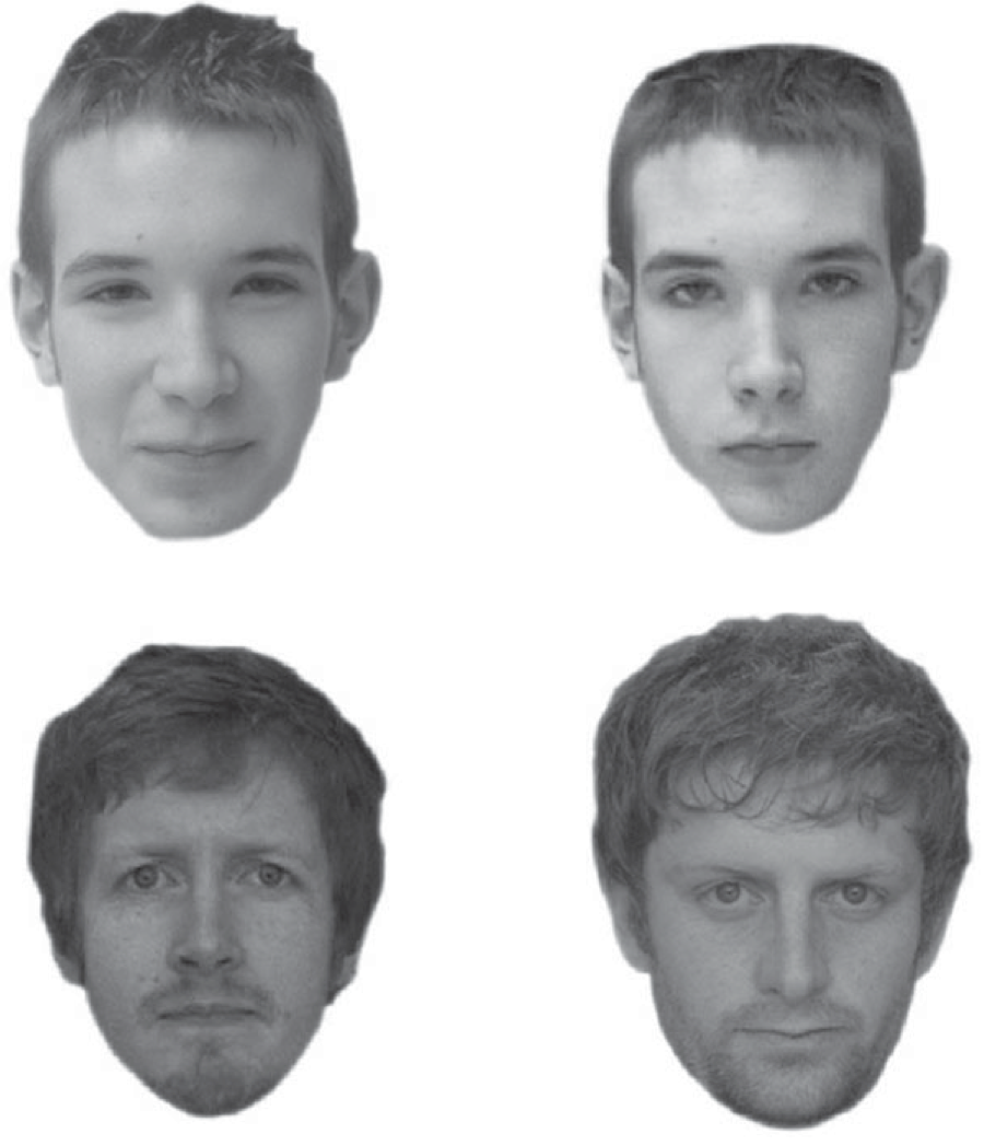
The top two pictures are the same person, the bottom two pictures are different people. For each pair of faces, the subject gets as much time as he or she needs and then says whether or not they are the same person. The subject then rates his or her confidence in the choice.
In this study, subjects also took surveys to determine properties about their sleep. The Sleep Condition Indicator (SCI) is a measure of insomnia disorder over the past month (scores of 16 and below indicate insomnia). The Pittsburgh Sleep Quality Index (PSQI) quantifies how well a subject sleeps in terms of interruptions, latency, etc. A higher score indicates poorer sleep. The Epworth Sleepiness Scale (ESS) assesses daytime drowsiness.
The data set is stored in the file ~/git/bootcamp/data/gfmt_sleep.csv. The contents of this file were adapted from the Excel file posted on the public Dryad repository. (Note this: if you want other people to use and explore your data, make it publicly available.)
This is a CSV file, where CSV stands for comma-separated value. This is a text file that is easily read into data structures in many programming languages. You should generally always store your data in such a format, not necessarily CSV, but a format that is open, has a well-defined specification, and is readable in many contexts. Excel files do not meet these criteria. Neither to .mat files.
Let’s take a look at the CSV file.
[2]:
!head data/gfmt_sleep.csv
participant number,gender,age,correct hit percentage,correct reject percentage,percent correct,confidence when correct hit,confidence when incorrect hit,confidence when correct reject,confidence when incorrect reject,confidence when correct,confidence when incorrect,sci,psqi,ess
8,f,39,65,80,72.5,91,90,93,83.5,93,90,9,13,2
16,m,42,90,90,90,75.5,55.5,70.5,50,75,50,4,11,7
18,f,31,90,95,92.5,89.5,90,86,81,89,88,10,9,3
22,f,35,100,75,87.5,89.5,*,71,80,88,80,13,8,20
27,f,74,60,65,62.5,68.5,49,61,49,65,49,13,9,12
28,f,61,80,20,50,71,63,31,72.5,64.5,70.5,15,14,2
30,m,32,90,75,82.5,67,56.5,66,65,66,64,16,9,3
33,m,62,45,90,67.5,54,37,65,81.5,62,61,14,9,9
34,f,33,80,100,90,70.5,76.5,64.5,*,68,76.5,14,12,10
The first line contains the headers for each column. They are participant number, gender, age, etc. The data follow. There are two important things to note here. First, notice that the gender column has string data (m or f), while the rest of the data are numeric. Note also that there are some missing data, denoted by the *s in the file.
Given the file I/O skills you recently learned, you could write some functions to parse this file and extract the data you want. You can imagine that this might be kind of painful. However, if the file format is nice and clean, like we more or less have here, we can use pre-built tools. Pandas has a very powerful function, pd.read_csv() that can read in a CSV file and store the contents in a convenient data structure called a data frame. In Pandas, the data type for a data frame is
DataFrame, and we will use “data frame” and “DataFrame” interchangeably.
Reading in data
Take a look at the doc string of pd.read_csv(). Holy cow! There are so many options we can specify for reading in a CSV file. You will likely find reasons to use many of these throughout your research. For this particular data set, we really only need the na_values kwarg. This specifies what characters signify that a data point is missing. The resulting data frame is populated with a NaN, or
not-a-number, wherever this character is present in the file. In this case, we want na_values='*'. So, let’s load in the data set.
[3]:
df = pd.read_csv('data/gfmt_sleep.csv', na_values='*')

# Check the type
type(df)
[3]:
pandas.core.frame.DataFrame
We now have the data stored in a data frame. We can look at it in the Jupyter notebook, since Jupyter will display it in a well-organized, pretty way.
[4]:
df
[4]:
| participant number | gender | age | correct hit percentage | correct reject percentage | percent correct | confidence when correct hit | confidence when incorrect hit | confidence when correct reject | confidence when incorrect reject | confidence when correct | confidence when incorrect | sci | psqi | ess | |
|---|---|---|---|---|---|---|---|---|---|---|---|---|---|---|---|
| 0 | 8 | f | 39 | 65 | 80 | 72.5 | 91.0 | 90.0 | 93.0 | 83.5 | 93.0 | 90.0 | 9 | 13 | 2 |
| 1 | 16 | m | 42 | 90 | 90 | 90.0 | 75.5 | 55.5 | 70.5 | 50.0 | 75.0 | 50.0 | 4 | 11 | 7 |
| 2 | 18 | f | 31 | 90 | 95 | 92.5 | 89.5 | 90.0 | 86.0 | 81.0 | 89.0 | 88.0 | 10 | 9 | 3 |
| 3 | 22 | f | 35 | 100 | 75 | 87.5 | 89.5 | NaN | 71.0 | 80.0 | 88.0 | 80.0 | 13 | 8 | 20 |
| 4 | 27 | f | 74 | 60 | 65 | 62.5 | 68.5 | 49.0 | 61.0 | 49.0 | 65.0 | 49.0 | 13 | 9 | 12 |
| ... | ... | ... | ... | ... | ... | ... | ... | ... | ... | ... | ... | ... | ... | ... | ... |
| 97 | 97 | f | 23 | 70 | 85 | 77.5 | 77.0 | 66.5 | 77.0 | 77.5 | 77.0 | 74.0 | 20 | 8 | 10 |
| 98 | 98 | f | 70 | 90 | 85 | 87.5 | 65.5 | 85.5 | 87.0 | 80.0 | 74.0 | 80.0 | 19 | 8 | 7 |
| 99 | 99 | f | 24 | 70 | 80 | 75.0 | 61.5 | 81.0 | 70.0 | 61.0 | 65.0 | 81.0 | 31 | 2 | 15 |
| 100 | 102 | f | 40 | 75 | 65 | 70.0 | 53.0 | 37.0 | 84.0 | 52.0 | 81.0 | 51.0 | 22 | 4 | 7 |
| 101 | 103 | f | 33 | 85 | 40 | 62.5 | 80.0 | 27.0 | 31.0 | 82.5 | 81.0 | 73.0 | 24 | 5 | 7 |
102 rows × 15 columns
This is a nice representation of the data, but we really do not need to display that many rows of the data frame in order to understand its structure. Instead, we can use the head() method of data frames to look at the first few rows.
[5]:
df.head()
[5]:
| participant number | gender | age | correct hit percentage | correct reject percentage | percent correct | confidence when correct hit | confidence when incorrect hit | confidence when correct reject | confidence when incorrect reject | confidence when correct | confidence when incorrect | sci | psqi | ess | |
|---|---|---|---|---|---|---|---|---|---|---|---|---|---|---|---|
| 0 | 8 | f | 39 | 65 | 80 | 72.5 | 91.0 | 90.0 | 93.0 | 83.5 | 93.0 | 90.0 | 9 | 13 | 2 |
| 1 | 16 | m | 42 | 90 | 90 | 90.0 | 75.5 | 55.5 | 70.5 | 50.0 | 75.0 | 50.0 | 4 | 11 | 7 |
| 2 | 18 | f | 31 | 90 | 95 | 92.5 | 89.5 | 90.0 | 86.0 | 81.0 | 89.0 | 88.0 | 10 | 9 | 3 |
| 3 | 22 | f | 35 | 100 | 75 | 87.5 | 89.5 | NaN | 71.0 | 80.0 | 88.0 | 80.0 | 13 | 8 | 20 |
| 4 | 27 | f | 74 | 60 | 65 | 62.5 | 68.5 | 49.0 | 61.0 | 49.0 | 65.0 | 49.0 | 13 | 9 | 12 |
This is more manageable and gives us an overview of what the columns are. Note also the the missing data was populated with NaN.
Indexing data frames
The data frame is a convenient data structure for many reasons that will become clear as we start exploring. Let’s start by looking at how data frames are indexed. Let’s try to look at the first row.
[6]:
df[0]
---------------------------------------------------------------------------
KeyError                                  Traceback (most recent call last)
File ~/opt/anaconda3/lib/python3.9/site-packages/pandas/core/indexes/base.py:3621, in Index.get_loc(self, key, method, tolerance)
   3620 try:
-> 3621     return self._engine.get_loc(casted_key)
   3622 except KeyError as err:

File ~/opt/anaconda3/lib/python3.9/site-packages/pandas/_libs/index.pyx:136, in pandas._libs.index.IndexEngine.get_loc()

File ~/opt/anaconda3/lib/python3.9/site-packages/pandas/_libs/index.pyx:163, in pandas._libs.index.IndexEngine.get_loc()

File pandas/_libs/hashtable_class_helper.pxi:5198, in pandas._libs.hashtable.PyObjectHashTable.get_item()

File pandas/_libs/hashtable_class_helper.pxi:5206, in pandas._libs.hashtable.PyObjectHashTable.get_item()

KeyError: 0

The above exception was the direct cause of the following exception:

KeyError                                  Traceback (most recent call last)
Input In [6], in <cell line: 1>()
----> 1 df[0]

File ~/opt/anaconda3/lib/python3.9/site-packages/pandas/core/frame.py:3505, in DataFrame.__getitem__(self, key)
   3503 if self.columns.nlevels > 1:
   3504     return self._getitem_multilevel(key)
-> 3505 indexer = self.columns.get_loc(key)
   3506 if is_integer(indexer):
   3507     indexer = [indexer]

File ~/opt/anaconda3/lib/python3.9/site-packages/pandas/core/indexes/base.py:3623, in Index.get_loc(self, key, method, tolerance)
   3621     return self._engine.get_loc(casted_key)
   3622 except KeyError as err:
-> 3623     raise KeyError(key) from err
   3624 except TypeError:
   3625     # If we have a listlike key, _check_indexing_error will raise
   3626     #  InvalidIndexError. Otherwise we fall through and re-raise
   3627     #  the TypeError.
   3628     self._check_indexing_error(key)

KeyError: 0
Yikes! Lots of errors. The problem is that we tried to index numerically by row. We index DataFrames by columns. And there is no column that has the name 0 in this data frame, though there could be. Instead, a might want to look at the column with the percentage of correct face matching tasks.
[7]:
df['percent correct']
[7]:
0      72.5
1      90.0
2      92.5
3      87.5
4      62.5
       ...
97     77.5
98     87.5
99     75.0
100    70.0
101    62.5
Name: percent correct, Length: 102, dtype: float64
This gave us the numbers we were after. Notice that when it was printed, the index of the rows came along with it. If we wanted to pull out a single percentage correct, say corresponding to index 4, we can do that.
[8]:
df['percent correct'][4]
[8]:
62.5
However, this is not the preferred way to do this. It is better to use .loc. This give the location in the data frame we want.
[9]:
df.loc[4, 'percent correct']
[9]:
62.5
Note that following .loc, we have the index by row then column, separated by a comma, in brackets. It is also important to note that row indices need not be integers. And you should not count on them being integers. In practice you will almost never use row indices, but rather use Boolean indexing.
Boolean indexing of data frames
Let’s say I wanted the percent correct of participant number 42. I can use Boolean indexing to specify the row. Specifically, I want the row for which df['participant number'] == 42. You can essentially plop this syntax directly when using .loc.
[10]:
df.loc[df['participant number'] == 42, 'percent correct']
[10]:
54    85.0
Name: percent correct, dtype: float64
If I want to pull the whole record for that participant, I can use : for the column index.
[11]:
df.loc[df['participant number'] == 42, :]
[11]:
| participant number | gender | age | correct hit percentage | correct reject percentage | percent correct | confidence when correct hit | confidence when incorrect hit | confidence when correct reject | confidence when incorrect reject | confidence when correct | confidence when incorrect | sci | psqi | ess | |
|---|---|---|---|---|---|---|---|---|---|---|---|---|---|---|---|
| 54 | 42 | m | 29 | 100 | 70 | 85.0 | 75.0 | NaN | 64.5 | 43.0 | 74.0 | 43.0 | 32 | 1 | 6 |
Notice that the index, 54, comes along for the ride, but we do not need it.
Now, let’s pull out all records of females under the age of 21. We can again use Boolean indexing, but we need to use an & operator. We did not cover this bitwise operator before, but the syntax is self-explanatory in the example below. Note that it is important that each Boolean operation you are doing is in parentheses because of the precedence of the operators involved.
[12]:
df.loc[(df['age'] < 21) & (df['gender'] == 'f'), :]
[12]:
| participant number | gender | age | correct hit percentage | correct reject percentage | percent correct | confidence when correct hit | confidence when incorrect hit | confidence when correct reject | confidence when incorrect reject | confidence when correct | confidence when incorrect | sci | psqi | ess | |
|---|---|---|---|---|---|---|---|---|---|---|---|---|---|---|---|
| 27 | 3 | f | 16 | 70 | 80 | 75.0 | 70.0 | 57.0 | 54.0 | 53.0 | 57.0 | 54.5 | 23 | 1 | 3 |
| 29 | 5 | f | 18 | 90 | 100 | 95.0 | 76.5 | 83.0 | 80.0 | NaN | 80.0 | 83.0 | 21 | 7 | 5 |
| 66 | 58 | f | 16 | 85 | 85 | 85.0 | 55.0 | 30.0 | 50.0 | 40.0 | 52.5 | 35.0 | 29 | 2 | 11 |
| 79 | 72 | f | 18 | 80 | 75 | 77.5 | 67.5 | 51.5 | 66.0 | 57.0 | 67.0 | 53.0 | 29 | 4 | 6 |
| 88 | 85 | f | 18 | 85 | 85 | 85.0 | 93.0 | 92.0 | 91.0 | 89.0 | 91.5 | 91.0 | 25 | 4 | 21 |
We can do something even more complicated, like pull out all females under 30 who got more than 85% of the face matching tasks correct. The code is clearer if we set up our Boolean indexing first, as follows.
[13]:
inds = (df["age"] < 30) & (df["gender"] == "f") & (df["percent correct"] > 85)

# Take a look
inds
[13]:
0      False
1      False
2      False
3      False
4      False
       ...
97     False
98     False
99     False
100    False
101    False
Length: 102, dtype: bool
Notice that inds is an array (actually a Pandas Series, essentially a DataFrame with one column) of Trues and Falses. When we index with it using .loc, we get back rows where inds is True.
[14]:
df.loc[inds, :]
[14]:
| participant number | gender | age | correct hit percentage | correct reject percentage | percent correct | confidence when correct hit | confidence when incorrect hit | confidence when correct reject | confidence when incorrect reject | confidence when correct | confidence when incorrect | sci | psqi | ess | |
|---|---|---|---|---|---|---|---|---|---|---|---|---|---|---|---|
| 22 | 93 | f | 28 | 100 | 75 | 87.5 | 89.5 | NaN | 67.0 | 60.0 | 80.0 | 60.0 | 16 | 7 | 4 |
| 29 | 5 | f | 18 | 90 | 100 | 95.0 | 76.5 | 83.0 | 80.0 | NaN | 80.0 | 83.0 | 21 | 7 | 5 |
| 30 | 6 | f | 28 | 95 | 80 | 87.5 | 100.0 | 85.0 | 94.0 | 61.0 | 99.0 | 65.0 | 19 | 7 | 12 |
| 33 | 10 | f | 25 | 100 | 100 | 100.0 | 90.0 | NaN | 85.0 | NaN | 90.0 | NaN | 17 | 10 | 11 |
| 56 | 44 | f | 21 | 85 | 90 | 87.5 | 66.0 | 29.0 | 70.0 | 29.0 | 67.0 | 29.0 | 26 | 7 | 18 |
| 58 | 48 | f | 23 | 90 | 85 | 87.5 | 67.0 | 47.0 | 69.0 | 40.0 | 67.0 | 40.0 | 18 | 6 | 8 |
| 60 | 51 | f | 24 | 85 | 95 | 90.0 | 97.0 | 41.0 | 74.0 | 73.0 | 83.0 | 55.5 | 29 | 1 | 7 |
| 75 | 67 | f | 25 | 100 | 100 | 100.0 | 61.5 | NaN | 58.5 | NaN | 60.5 | NaN | 28 | 8 | 9 |
Of interest in this exercise in Boolean indexing is that we never had to write a loop. To produce our indices, we could have done the following.
[15]:
# Initialize array of Boolean indices
inds = [False] * len(df)

# Iterate over the rows of the DataFrame to check if the row should be included
for i, r in df.iterrows():
    if r['age'] < 30 and r['gender'] == 'f' and r['percent correct'] > 85:
        inds[i] = True

# Make our seleciton with Boolean indexing
df.loc[inds, :]
[15]:
| participant number | gender | age | correct hit percentage | correct reject percentage | percent correct | confidence when correct hit | confidence when incorrect hit | confidence when correct reject | confidence when incorrect reject | confidence when correct | confidence when incorrect | sci | psqi | ess | |
|---|---|---|---|---|---|---|---|---|---|---|---|---|---|---|---|
| 22 | 93 | f | 28 | 100 | 75 | 87.5 | 89.5 | NaN | 67.0 | 60.0 | 80.0 | 60.0 | 16 | 7 | 4 |
| 29 | 5 | f | 18 | 90 | 100 | 95.0 | 76.5 | 83.0 | 80.0 | NaN | 80.0 | 83.0 | 21 | 7 | 5 |
| 30 | 6 | f | 28 | 95 | 80 | 87.5 | 100.0 | 85.0 | 94.0 | 61.0 | 99.0 | 65.0 | 19 | 7 | 12 |
| 33 | 10 | f | 25 | 100 | 100 | 100.0 | 90.0 | NaN | 85.0 | NaN | 90.0 | NaN | 17 | 10 | 11 |
| 56 | 44 | f | 21 | 85 | 90 | 87.5 | 66.0 | 29.0 | 70.0 | 29.0 | 67.0 | 29.0 | 26 | 7 | 18 |
| 58 | 48 | f | 23 | 90 | 85 | 87.5 | 67.0 | 47.0 | 69.0 | 40.0 | 67.0 | 40.0 | 18 | 6 | 8 |
| 60 | 51 | f | 24 | 85 | 95 | 90.0 | 97.0 | 41.0 | 74.0 | 73.0 | 83.0 | 55.5 | 29 | 1 | 7 |
| 75 | 67 | f | 25 | 100 | 100 | 100.0 | 61.5 | NaN | 58.5 | NaN | 60.5 | NaN | 28 | 8 | 9 |
This feature, where the looping is done automatically on Pandas objects like data frames, is very powerful and saves us writing lots of lines of code. This example also showed how to use the iterrows() method of a data frame to iterate over the rows of a data frame. It is actually rare that you will need to do that, as we’ll show next when computing with data frames.
Calculating with data frames
Recall that a subject is said to suffer from insomnia if he or she has an SCI of 16 or below. We might like to add a column to the data frame that specifies whether or not the subject suffers from insomnia. We can conveniently compute with columns. This is done elementwise.
[16]:
df['sci'] <= 16
[16]:
0       True
1       True
2       True
3       True
4       True
       ...
97     False
98     False
99     False
100    False
101    False
Name: sci, Length: 102, dtype: bool
This tells use who is an insomniac. We can simply add this back to the data frame.
[17]:
# Add the column to the DataFrame
df['insomnia'] = df['sci'] <= 16

# Take a look
df.head()
[17]:
| participant number | gender | age | correct hit percentage | correct reject percentage | percent correct | confidence when correct hit | confidence when incorrect hit | confidence when correct reject | confidence when incorrect reject | confidence when correct | confidence when incorrect | sci | psqi | ess | insomnia | |
|---|---|---|---|---|---|---|---|---|---|---|---|---|---|---|---|---|
| 0 | 8 | f | 39 | 65 | 80 | 72.5 | 91.0 | 90.0 | 93.0 | 83.5 | 93.0 | 90.0 | 9 | 13 | 2 | True |
| 1 | 16 | m | 42 | 90 | 90 | 90.0 | 75.5 | 55.5 | 70.5 | 50.0 | 75.0 | 50.0 | 4 | 11 | 7 | True |
| 2 | 18 | f | 31 | 90 | 95 | 92.5 | 89.5 | 90.0 | 86.0 | 81.0 | 89.0 | 88.0 | 10 | 9 | 3 | True |
| 3 | 22 | f | 35 | 100 | 75 | 87.5 | 89.5 | NaN | 71.0 | 80.0 | 88.0 | 80.0 | 13 | 8 | 20 | True |
| 4 | 27 | f | 74 | 60 | 65 | 62.5 | 68.5 | 49.0 | 61.0 | 49.0 | 65.0 | 49.0 | 13 | 9 | 12 | True |
A note about vectorization
Notice how applying the <= operator to a Series resulted in elementwise application. This is called vectorization. It means that we do not have to write a for loop to do operations on the elements of a Series or other array-like object. Imagine if we had to do that with a for loop.
[18]:
insomnia = []
for sci in df['sci']:
    insomnia.append(sci <= 16)
This is cumbersome. The vectorization allows for much more convenient calculation. Beyond that, the vectorized code is almost always faster when using Pandas and Numpy because the looping is done with compiled code under the hood. This can be done with many operators, including those you’ve already seen, like +, -, *, /, **, etc.
Applying functions to Pandas objects
Remember when we briefly saw the np.mean() function? We can compute with that as well. Let’s compare the mean percent correct for insomniacs versus those who are not.
[19]:
print('Insomniacs:', np.mean(df.loc[df['insomnia'], 'percent correct']))
print('Control:   ', np.mean(df.loc[~df['insomnia'], 'percent correct']))
Insomniacs: 76.1
Control:    81.46103896103897
Notice that I used the ~ operator, which is a bit switcher. It changes all Trues to Falses and vice versa. In this case, it functions like a logical NOT.
We will do a lot more computing with Pandas data frames in the next lessons. For our last demonstration in this lesson, we can quickly compute summary statistics about each column of a data frame using its describe() method.
[20]:
df.describe()
[20]:
| participant number | age | correct hit percentage | correct reject percentage | percent correct | confidence when correct hit | confidence when incorrect hit | confidence when correct reject | confidence when incorrect reject | confidence when correct | confidence when incorrect | sci | psqi | ess | |
|---|---|---|---|---|---|---|---|---|---|---|---|---|---|---|
| count | 102.000000 | 102.000000 | 102.000000 | 102.000000 | 102.000000 | 102.000000 | 84.000000 | 102.000000 | 93.000000 | 102.000000 | 99.000000 | 102.000000 | 102.000000 | 102.000000 |
| mean | 52.049020 | 37.921569 | 83.088235 | 77.205882 | 80.147059 | 74.990196 | 58.565476 | 71.137255 | 61.220430 | 74.642157 | 61.979798 | 22.245098 | 5.274510 | 7.294118 |
| std | 30.020909 | 14.029450 | 15.091210 | 17.569854 | 12.047881 | 14.165916 | 19.560653 | 14.987479 | 17.671283 | 13.619725 | 15.921670 | 7.547128 | 3.404007 | 4.426715 |
| min | 1.000000 | 16.000000 | 35.000000 | 20.000000 | 40.000000 | 29.500000 | 7.000000 | 19.000000 | 17.000000 | 24.000000 | 24.500000 | 0.000000 | 0.000000 | 0.000000 |
| 25% | 26.250000 | 26.500000 | 75.000000 | 70.000000 | 72.500000 | 66.000000 | 46.375000 | 64.625000 | 50.000000 | 66.000000 | 51.000000 | 17.000000 | 3.000000 | 4.000000 |
| 50% | 52.500000 | 36.500000 | 90.000000 | 80.000000 | 83.750000 | 75.000000 | 56.250000 | 71.250000 | 61.000000 | 75.750000 | 61.500000 | 23.500000 | 5.000000 | 7.000000 |
| 75% | 77.750000 | 45.000000 | 95.000000 | 90.000000 | 87.500000 | 86.500000 | 73.500000 | 80.000000 | 74.000000 | 82.375000 | 73.000000 | 29.000000 | 7.000000 | 10.000000 |
| max | 103.000000 | 74.000000 | 100.000000 | 100.000000 | 100.000000 | 100.000000 | 92.000000 | 100.000000 | 100.000000 | 100.000000 | 100.000000 | 32.000000 | 15.000000 | 21.000000 |
This gives us a data frame with summary statistics. Note that in this data frame, the row indices are not integers, but are the names of the summary statistics. If we wanted to extract the median value of each entry, we could do that with .loc.
[21]:
df.describe().loc['50%', :]
[21]:
participant number                  52.50
age                                 36.50
correct hit percentage              90.00
correct reject percentage           80.00
percent correct                     83.75
confidence when correct hit         75.00
confidence when incorrect hit       56.25
confidence when correct reject      71.25
confidence when incorrect reject    61.00
confidence when correct             75.75
confidence when incorrect           61.50
sci                                 23.50
psqi                                 5.00
ess                                  7.00
Name: 50%, dtype: float64
Outputting a new CSV file
Now that we added the insomniac column, we might like to save our data frame as a new CSV that we can reload later. We use df.to_csv() for this with the index kwarg to ask Pandas not to explicitly write the indices to the file.
[22]:
df.to_csv('gfmt_sleep_with_insomnia.csv', index=False)
Let’s take a look at what this file looks like.
[23]:
!head gfmt_sleep_with_insomnia.csv
participant number,gender,age,correct hit percentage,correct reject percentage,percent correct,confidence when correct hit,confidence when incorrect hit,confidence when correct reject,confidence when incorrect reject,confidence when correct,confidence when incorrect,sci,psqi,ess,insomnia
8,f,39,65,80,72.5,91.0,90.0,93.0,83.5,93.0,90.0,9,13,2,True
16,m,42,90,90,90.0,75.5,55.5,70.5,50.0,75.0,50.0,4,11,7,True
18,f,31,90,95,92.5,89.5,90.0,86.0,81.0,89.0,88.0,10,9,3,True
22,f,35,100,75,87.5,89.5,,71.0,80.0,88.0,80.0,13,8,20,True
27,f,74,60,65,62.5,68.5,49.0,61.0,49.0,65.0,49.0,13,9,12,True
28,f,61,80,20,50.0,71.0,63.0,31.0,72.5,64.5,70.5,15,14,2,True
30,m,32,90,75,82.5,67.0,56.5,66.0,65.0,66.0,64.0,16,9,3,True
33,m,62,45,90,67.5,54.0,37.0,65.0,81.5,62.0,61.0,14,9,9,True
34,f,33,80,100,90.0,70.5,76.5,64.5,,68.0,76.5,14,12,10,True
Very nice. Notice that by default Pandas leaves an empty field for NaNs, and we do not need the na_values kwarg when we load in this CSV file.
Styling a data frame
It is sometimes useful to highlight features in a data frame when viewing them. (Note that this is generally far less useful than making informative plots, which we will come to shortly.) Pandas offers some convenient ways to style the display of a data frame.
As an example, let’s say we wanted to highlight rows corresponding to women who scored at or above 75% correct. We can write a function that will take as an argument a row of the data frame, check the value in the 'gender' and 'percent correct' columns, and then specify a row color of gray or green accordingly. We then use df.style.apply() with the axis=1 kwarg to apply that function to each row.
[24]:
def highlight_high_scoring_females(s):
    if s["gender"] == "f" and s["percent correct"] >= 75:
        return ["background-color: #7fc97f"] * len(s)
    else:
        return ["background-color: lightgray"] * len(s)

df.head(10).style.apply(highlight_high_scoring_females, axis=1)
[24]:
| participant number | gender | age | correct hit percentage | correct reject percentage | percent correct | confidence when correct hit | confidence when incorrect hit | confidence when correct reject | confidence when incorrect reject | confidence when correct | confidence when incorrect | sci | psqi | ess | insomnia | |
|---|---|---|---|---|---|---|---|---|---|---|---|---|---|---|---|---|
| 0 | 8 | f | 39 | 65 | 80 | 72.500000 | 91.000000 | 90.000000 | 93.000000 | 83.500000 | 93.000000 | 90.000000 | 9 | 13 | 2 | True |
| 1 | 16 | m | 42 | 90 | 90 | 90.000000 | 75.500000 | 55.500000 | 70.500000 | 50.000000 | 75.000000 | 50.000000 | 4 | 11 | 7 | True |
| 2 | 18 | f | 31 | 90 | 95 | 92.500000 | 89.500000 | 90.000000 | 86.000000 | 81.000000 | 89.000000 | 88.000000 | 10 | 9 | 3 | True |
| 3 | 22 | f | 35 | 100 | 75 | 87.500000 | 89.500000 | nan | 71.000000 | 80.000000 | 88.000000 | 80.000000 | 13 | 8 | 20 | True |
| 4 | 27 | f | 74 | 60 | 65 | 62.500000 | 68.500000 | 49.000000 | 61.000000 | 49.000000 | 65.000000 | 49.000000 | 13 | 9 | 12 | True |
| 5 | 28 | f | 61 | 80 | 20 | 50.000000 | 71.000000 | 63.000000 | 31.000000 | 72.500000 | 64.500000 | 70.500000 | 15 | 14 | 2 | True |
| 6 | 30 | m | 32 | 90 | 75 | 82.500000 | 67.000000 | 56.500000 | 66.000000 | 65.000000 | 66.000000 | 64.000000 | 16 | 9 | 3 | True |
| 7 | 33 | m | 62 | 45 | 90 | 67.500000 | 54.000000 | 37.000000 | 65.000000 | 81.500000 | 62.000000 | 61.000000 | 14 | 9 | 9 | True |
| 8 | 34 | f | 33 | 80 | 100 | 90.000000 | 70.500000 | 76.500000 | 64.500000 | nan | 68.000000 | 76.500000 | 14 | 12 | 10 | True |
| 9 | 35 | f | 53 | 100 | 50 | 75.000000 | 74.500000 | nan | 60.500000 | 65.000000 | 71.000000 | 65.000000 | 14 | 8 | 7 | True |
We can be more fancy. Let’s say we want to shade the 'percent correct' column with a bar corresponding to the value in the column. We use the df.style.bar() method to do so. The subset kwarg specifies which columns are to have bars.
[25]:
df.head(10).style.bar(subset=["percent correct"], vmin=0, vmax=100)
[25]:
| participant number | gender | age | correct hit percentage | correct reject percentage | percent correct | confidence when correct hit | confidence when incorrect hit | confidence when correct reject | confidence when incorrect reject | confidence when correct | confidence when incorrect | sci | psqi | ess | insomnia | |
|---|---|---|---|---|---|---|---|---|---|---|---|---|---|---|---|---|
| 0 | 8 | f | 39 | 65 | 80 | 72.500000 | 91.000000 | 90.000000 | 93.000000 | 83.500000 | 93.000000 | 90.000000 | 9 | 13 | 2 | True |
| 1 | 16 | m | 42 | 90 | 90 | 90.000000 | 75.500000 | 55.500000 | 70.500000 | 50.000000 | 75.000000 | 50.000000 | 4 | 11 | 7 | True |
| 2 | 18 | f | 31 | 90 | 95 | 92.500000 | 89.500000 | 90.000000 | 86.000000 | 81.000000 | 89.000000 | 88.000000 | 10 | 9 | 3 | True |
| 3 | 22 | f | 35 | 100 | 75 | 87.500000 | 89.500000 | nan | 71.000000 | 80.000000 | 88.000000 | 80.000000 | 13 | 8 | 20 | True |
| 4 | 27 | f | 74 | 60 | 65 | 62.500000 | 68.500000 | 49.000000 | 61.000000 | 49.000000 | 65.000000 | 49.000000 | 13 | 9 | 12 | True |
| 5 | 28 | f | 61 | 80 | 20 | 50.000000 | 71.000000 | 63.000000 | 31.000000 | 72.500000 | 64.500000 | 70.500000 | 15 | 14 | 2 | True |
| 6 | 30 | m | 32 | 90 | 75 | 82.500000 | 67.000000 | 56.500000 | 66.000000 | 65.000000 | 66.000000 | 64.000000 | 16 | 9 | 3 | True |
| 7 | 33 | m | 62 | 45 | 90 | 67.500000 | 54.000000 | 37.000000 | 65.000000 | 81.500000 | 62.000000 | 61.000000 | 14 | 9 | 9 | True |
| 8 | 34 | f | 33 | 80 | 100 | 90.000000 | 70.500000 | 76.500000 | 64.500000 | nan | 68.000000 | 76.500000 | 14 | 12 | 10 | True |
| 9 | 35 | f | 53 | 100 | 50 | 75.000000 | 74.500000 | nan | 60.500000 | 65.000000 | 71.000000 | 65.000000 | 14 | 8 | 7 | True |
Note that I have used the vmin=0 and vmax=100 kwargs to set the base of the bar to be at zero and the maximum to be 100.
Alternatively, I could color the percent correct according to the percent correct.
[26]:
df.head(10).style.background_gradient(subset=["percent correct"], cmap="Reds")
[26]:
| participant number | gender | age | correct hit percentage | correct reject percentage | percent correct | confidence when correct hit | confidence when incorrect hit | confidence when correct reject | confidence when incorrect reject | confidence when correct | confidence when incorrect | sci | psqi | ess | insomnia | |
|---|---|---|---|---|---|---|---|---|---|---|---|---|---|---|---|---|
| 0 | 8 | f | 39 | 65 | 80 | 72.500000 | 91.000000 | 90.000000 | 93.000000 | 83.500000 | 93.000000 | 90.000000 | 9 | 13 | 2 | True |
| 1 | 16 | m | 42 | 90 | 90 | 90.000000 | 75.500000 | 55.500000 | 70.500000 | 50.000000 | 75.000000 | 50.000000 | 4 | 11 | 7 | True |
| 2 | 18 | f | 31 | 90 | 95 | 92.500000 | 89.500000 | 90.000000 | 86.000000 | 81.000000 | 89.000000 | 88.000000 | 10 | 9 | 3 | True |
| 3 | 22 | f | 35 | 100 | 75 | 87.500000 | 89.500000 | nan | 71.000000 | 80.000000 | 88.000000 | 80.000000 | 13 | 8 | 20 | True |
| 4 | 27 | f | 74 | 60 | 65 | 62.500000 | 68.500000 | 49.000000 | 61.000000 | 49.000000 | 65.000000 | 49.000000 | 13 | 9 | 12 | True |
| 5 | 28 | f | 61 | 80 | 20 | 50.000000 | 71.000000 | 63.000000 | 31.000000 | 72.500000 | 64.500000 | 70.500000 | 15 | 14 | 2 | True |
| 6 | 30 | m | 32 | 90 | 75 | 82.500000 | 67.000000 | 56.500000 | 66.000000 | 65.000000 | 66.000000 | 64.000000 | 16 | 9 | 3 | True |
| 7 | 33 | m | 62 | 45 | 90 | 67.500000 | 54.000000 | 37.000000 | 65.000000 | 81.500000 | 62.000000 | 61.000000 | 14 | 9 | 9 | True |
| 8 | 34 | f | 33 | 80 | 100 | 90.000000 | 70.500000 | 76.500000 | 64.500000 | nan | 68.000000 | 76.500000 | 14 | 12 | 10 | True |
| 9 | 35 | f | 53 | 100 | 50 | 75.000000 | 74.500000 | nan | 60.500000 | 65.000000 | 71.000000 | 65.000000 | 14 | 8 | 7 | True |
We could have multiple effects together as well.
[27]:
df.head(10).style.bar(
    subset=["percent correct"], vmin=0, vmax=100
).apply(
    highlight_high_scoring_females, axis=1
)
[27]:
| participant number | gender | age | correct hit percentage | correct reject percentage | percent correct | confidence when correct hit | confidence when incorrect hit | confidence when correct reject | confidence when incorrect reject | confidence when correct | confidence when incorrect | sci | psqi | ess | insomnia | |
|---|---|---|---|---|---|---|---|---|---|---|---|---|---|---|---|---|
| 0 | 8 | f | 39 | 65 | 80 | 72.500000 | 91.000000 | 90.000000 | 93.000000 | 83.500000 | 93.000000 | 90.000000 | 9 | 13 | 2 | True |
| 1 | 16 | m | 42 | 90 | 90 | 90.000000 | 75.500000 | 55.500000 | 70.500000 | 50.000000 | 75.000000 | 50.000000 | 4 | 11 | 7 | True |
| 2 | 18 | f | 31 | 90 | 95 | 92.500000 | 89.500000 | 90.000000 | 86.000000 | 81.000000 | 89.000000 | 88.000000 | 10 | 9 | 3 | True |
| 3 | 22 | f | 35 | 100 | 75 | 87.500000 | 89.500000 | nan | 71.000000 | 80.000000 | 88.000000 | 80.000000 | 13 | 8 | 20 | True |
| 4 | 27 | f | 74 | 60 | 65 | 62.500000 | 68.500000 | 49.000000 | 61.000000 | 49.000000 | 65.000000 | 49.000000 | 13 | 9 | 12 | True |
| 5 | 28 | f | 61 | 80 | 20 | 50.000000 | 71.000000 | 63.000000 | 31.000000 | 72.500000 | 64.500000 | 70.500000 | 15 | 14 | 2 | True |
| 6 | 30 | m | 32 | 90 | 75 | 82.500000 | 67.000000 | 56.500000 | 66.000000 | 65.000000 | 66.000000 | 64.000000 | 16 | 9 | 3 | True |
| 7 | 33 | m | 62 | 45 | 90 | 67.500000 | 54.000000 | 37.000000 | 65.000000 | 81.500000 | 62.000000 | 61.000000 | 14 | 9 | 9 | True |
| 8 | 34 | f | 33 | 80 | 100 | 90.000000 | 70.500000 | 76.500000 | 64.500000 | nan | 68.000000 | 76.500000 | 14 | 12 | 10 | True |
| 9 | 35 | f | 53 | 100 | 50 | 75.000000 | 74.500000 | nan | 60.500000 | 65.000000 | 71.000000 | 65.000000 | 14 | 8 | 7 | True |
In practice, I almost never use these features because it is almost always better to display results as a plot rather than in tabular form. Still, it can be useful when exploring data sets to highlight certain aspects in tabular form.
Computing environment
[28]:
%load_ext watermark
%watermark -v -p numpy,pandas,jupyterlab
Python implementation: CPython
Python version       : 3.9.12
IPython version      : 8.3.0

numpy     : 1.21.5
pandas    : 1.4.2
jupyterlab: 3.3.2