Lesson 18: Plotting time series and generated data

---

import numpy as np
import pandas as pd
import scipy.special

import bokeh.io
import bokeh.plotting

bokeh.io.output_notebook()

Loading BokehJS ...

---

So far, we have only seen how to plot measured data. We have make plots using Bokeh where each glyph represents a single measurement. We used some glyphs that did not represent singe measurements when we make box plots, histograms, and formal (staircase-like) ECDFs, but the construction of those plots was abstracted away in the Bokeh-catplot package. In this lesson, we will learn how to make plots where the points are related to one another via an ordering so that we can connect the points with lines. It is one extra aspect to think about when constructing a graphic.

Plotting time series data

One class of measured data we have not considered is time series data. Time series data are typically not plotted as points, but rather with joined lines. To get some experience plotting data sets like this, we will use some data from Markus Meister’s group, collected by Dawna Bagherian and Kyu Lee. The file ~/git/bootcamp/data/retina_spikes.csv contains the data set. They put electrodes in the retinal cells of a mouse and measured voltage. From the time trace of voltage, they can detect and characterize spiking events. The first column of the CSV file is the time in milliseconds (ms) that the measurement was taken, and the second column is the voltage in units of microvolts (µV). Let’s load in the data.

df = pd.read_csv('data/retina_spikes.csv', comment='#')

df.head()

	t (ms)	V (uV)
0	703.96	4.79
1	704.00	-0.63
2	704.04	5.83
3	704.08	0.31
4	704.12	-4.58

Let’s create a figure to hold our plot. We will make it wide and narrow, since it is a long time course of potentials.

p = bokeh.plotting.figure(
    frame_height=150,
    frame_width=600,
    toolbar_location='above',
    x_axis_label='t (ms)',
    y_axis_label='V (µV)'
)

To make a plot of these data, we use the p.line() method. This makes a line with joints at each measurement. I always use the line_join='bevel' kwarg because the default joining of the line ('mitre') results in sharp corners. I also usually choose line_width=2, giving me a line two pixels in width, since I find the default of one pixel to be a bit thin. You can check out the available line properties in the Bokeh docs.

p.line(
    source=df,
    x='t (ms)',
    y='V (uV)',
    line_join='bevel',
    line_width=2,
)

bokeh.io.show(p)

We can clearly see several spiking events in the data. When we zoom, we can resolve the finer structure.

Plotting generated data

You’re now a pro at plotting measured data. But sometimes, you want to plot smooth functions. To do this, you can use Numpy and/or Scipy to generate arrays of values of smooth functions.

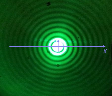
We will plot the Airy disk, which we encounter in biology when doing microscopy as the diffraction pattern of light passing through a pinhole. Here is a picture of the diffraction pattern from a laser (with the main peak overexposed).

The equation for the radial light intensity of an Airy disk is

\begin{align} \frac{I(x)}{I_0} = 4 \left(\frac{J_1(x)}{x}\right)^2, \end{align}

where \(I_0\) is the maximum intensity (the intensity at the center of the image) and \(x\) is the radial distance from the center. Here, \(J_1(x)\) is the first order Bessel function of the first kind. Yeesh. How do we plot that?

Fortunately, SciPy has lots of special functions available. Specifically, scipy.special.j1() computes exactly what we are after! We pass in a NumPy array that has the values of \(x\) we want to plot and then compute the \(y\)-values using the expression for the normalized intensity.

To plot a smooth curve, we use the np.linspace() function with lots of points. We then connect the points with straight lines, which to the eye look like a smooth curve. Let’s try it. We’ll use 400 points, which I find is a good rule of thumb for not-too-oscillating functions.

# The x-values we want
x = np.linspace(-15, 15, 400)

# The normalized intensity
norm_I = 4 * (scipy.special.j1(x) / x)**2

Now that we have the values we want to plot, we could construct a Pandas DataFrame to pass in as the source to p.line(). We do not need to take this extra step, though. If we instead leave source unspecified, and pass in NumPy arrays for x and y, Bokeh will directly use those in constructing the plot.

p = bokeh.plotting.figure(
    frame_height=250,
    frame_width=550,
    x_axis_label='x',
    y_axis_label='I(x)/I₀',
)

p.line(
    x=x,
    y=norm_I,
    line_join='bevel',
    line_width=2,
)

bokeh.io.show(p)

We could also plot dots (which doesn’t make sense here, but we’ll show it just to see who the line joining works to make a plot of a smooth function).

p.circle(
    x=x,
    y=norm_I,
    size=2,
    color='orange'
)

bokeh.io.show(p)

There is one detail I swept under the rug here. What happens if we compute the function for \(x = 0\)?

4 * (scipy.special.j1(0) / 0)**2

/Users/bois/opt/anaconda3/lib/python3.7/site-packages/ipykernel_launcher.py:1: RuntimeWarning: invalid value encountered in double_scalars
  """Entry point for launching an IPython kernel.

nan

We get a RuntimeWarning because we divided by zero. We know that

\begin{align} \lim_{x\to 0} \frac{J_1(x)}{x} = \frac{1}{2}, \end{align}

so we could write a new function that checks if \(x = 0\) and returns the appropriate limit for \(x = 0\). In the x array I constructed for the plot, we hopped over zero, so it was never evaluated. If we were being careful, we could write our own Airy function that deals with this.

def airy_disk(x):
    """Compute the Airy disk."""
    # Set up output array
    res = np.empty_like(x)

    # Where x is very close to zero (use np.isclose)
    near_zero = np.isclose(x, 0)

    # Compute values where x is close to zero
    res[near_zero] = 1.0

    # Everywhere else
    x_vals = x[~near_zero]
    res[~near_zero] = 4 * (scipy.special.j1(x_vals) / x_vals)**2

    return res

Computing environment

%load_ext watermark
%watermark -v -p numpy,scipy,pandas,bokeh,jupyterlab

CPython 3.7.7
IPython 7.13.0

numpy 1.18.1
scipy 1.4.1
pandas 0.24.2
bokeh 2.0.2
jupyterlab 1.2.6