Exercise 4.4: Monte Carlo simulation of transcriptional pausing

In this exercise, we will put random number generation to use and do a Monte Carlo simulation. The term Monte Carlo simulation is a broad term describing techniques in which a large number of random numbers are generated to (approximately) calculate properties of probability distributions. In many cases the analytical form of these distributions is not known, so Monte Carlo methods are a great way to learn about them.

Transcription, the process by which DNA is transcribed into RNA, is key process in the central dogma of molecular biology. RNA polymerase (RNAP) is at the heart of this process. This amazing machine glides along the DNA template, unzipping it internally, incorporating ribonucleotides at the front, and spitting RNA out the back. Sometimes, though, the polymerase pauses and then backtracks, pushing the RNA transcript back out the front, as shown in the figure below, taken from Depken, et al., Biophys. J., 96, 2189-2193, 2009.

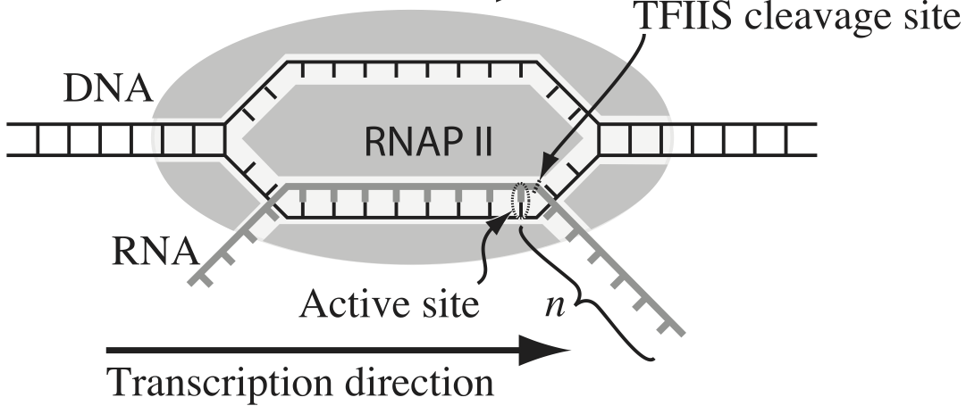
To escape these backtracks, a cleavage enzyme called TFIIS cleaves the bit on RNA hanging out of the front, and the RNAP can then go about its merry way.

Researchers have long debated how these backtracks are governed. Single molecule experiments can provide some much needed insight. The groups of Carlos Bustamante, Steve Block, and Stephan Grill, among others, have investigated the dynamics of RNAP in the absence of TFIIS. They can measure many individual backtracks and get statistics about how long the backtracks last.

One hypothesis is that the backtracks simply consist of diffusive-like motion along the DNA stand. That is to say, the polymerase can move forward or backward along the strand with equal probability once it is paused. This is a one-dimensional random walk. So, if we want to test this hypothesis, we would want to know how much time we should expect the RNAP to be in a backtrack so that we could compare to experiment.

So, we seek the probability distribution of backtrack times, \(P(t_{bt})\), where \(t_{bt}\) is the time spent in the backtrack. We could solve this analytically, which requires some sophisticated mathematics. But, because we know how to draw random numbers, we can just compute this distribution directly using Monte Carlo simulation!

We start at \(x = 0\) at time \(t = 0\). We “flip a coin,” or choose a random number to decide whether we step left or right. We do this again and again, keeping track of how many steps we take and what the \(x\) position is. As soon as \(x\) becomes positive, we have existed the backtrack. The total time for a backtrack is then \(\tau n_\mathrm{steps}\), where \(\tau\) is the time it takes to make a step. Depken, et al., report that \(\tau \approx 0.5\) seconds.

a) Write a function, backtrack_steps(), that computes the number of steps it takes for a random walker (i.e., polymerase) starting at position \(x = 0\) to get to position \(x = +1\). It should return the number of steps to take the walk.

b) Generate 10,000 of these backtracks in order to get enough samples out of \(P(t_\mathrm{bt})\). Some of these samples may take a very long time to acquire. (If you are interested in a way to really speed up this calculation, ask me about Numba. If you do use Numba, note that you must use the standard Mersenne Twister RNG for Numba; that is using np.random.....)

c) Generate an ECDF of your samples and plot the ECDF with the \(x\) axis on a logarithmic scale.

d) A probability distribution function that obeys a power law has the property

\begin{align} P(t_\mathrm{bt}) \propto t_\mathrm{bt}^{-a} \end{align}

in some part of the distribution, usually for large \(t_\mathrm{bt}\). If this is the case, the cumulative distribution function is then

\begin{align} \mathrm{CDF}(t_\mathrm{bt}) \equiv F(t_\mathrm{bt})= \int_{-\infty}^{t_\mathrm{bt}} \mathrm{d}t_\mathrm{bt}'\,P(t_\mathrm{bt}') = 1 - \frac{c}{t_\mathrm{bt}^{a+1}}, \end{align}

where \(c\) is some constant defined by the functional form of \(P(t_\mathrm{bt})\) for small \(t_\mathrm{bt}\) and the normalization condition. If \(F\) is our cumulative histogram, we can check for power law behavior by plotting the complementary cumulative distribution (CCDF), \(1 - F\), versus \(t_\mathrm{bt}\). If a power law is in play, the plot will be linear on a log-log scale with a slope of \(-a+1\).

Plot the complementary cumulative distribution function from your samples on a log-log plot. If it is linear, then the time to exit a backtrack is a power law.

e) By doing some mathematical heavy lifting, we know that, in the limit of large \(t_{bt}\),

\begin{align} P(t_{bt}) \propto t_{bt}^{-3/2}, \end{align}

so the plot you did in part (e) should have a slope of \(-1/2\) on a log-log plot. Is this what you see?

Notes: The theory to derive the probability distribution is involved. See, e.g., this. However, we were able to predict that we would see a great many short backtracks, and then see some very very long backtracks because of the power law distribution of backtrack times. We were able to do that just by doing a simple Monte Carlo simulation with “coin flips”. There are many problems where the theory is really hard, and deriving the distribution is currently impossible, or the probability distribution has such an ugly expression that we can’t really work with it. So, Monte Carlo methods are a powerful tool for generating predictions from simply-stated, but mathematically challenging, hypotheses.

Interestingly, many researchers thought (and maybe still do) there were two classes of backtracks: long and short. There may be, but the hypothesis that the backtrack is a random walk process is commensurate with seeing both very long and very short backtracks.

Solution

[1]:

import tqdm

import numpy as np
import numba

import iqplot

import bokeh.io
import bokeh.plotting

bokeh.io.output_notebook()

Loading BokehJS ...

a) For speed, I will use Numba to compile the function. You can read more about Numba here. For now, though, you can just ignore the @numba.njit decorator on the function.

[2]:

@numba.njit
def backtrack_steps():
    """
    Compute the number of steps it takes a 1d random walker starting
    at zero to get to +1.
    """
    # Initialize position and number of steps
    x = 0
    n_steps = 0

    # Walk until we get to positive 1
    while x < 1:
        x += 2 * np.random.randint(0, 2) - 1
        n_steps += 1

    return n_steps

b) Now let’s run it lots and lots of times. We will convert the result to time using the fact that each step takes about half a second.

When we run multiple simulations, it might be nice to have a progress bar. The tqdm module allows you to easily set up progress bars. To use it, just surround any iterator in a for loop with tqdm.tqdm(). For example, you could do:

for i in tqdm.tqdm(range(10000)):

[3]:

# Stepping time
tau = 0.5 # seconds

# Specify number of samples
n_samples = 10000

# Array of backtrack times
t_bt = np.empty(n_samples)

# Generate the samples
for i in tqdm.tqdm(range(n_samples)):
    t_bt[i] = backtrack_steps()

# Convert to seconds
t_bt *= tau

100%|████████████████████████████████████| 10000/10000 [00:15<00:00, 663.31it/s]

c) Now, let’s plot an ECDF of our backtrack times.

[4]:

p = iqplot.ecdf(
    t_bt,
    q='time of backtrack (s)',
    x_axis_type='log',
)

bokeh.io.show(p)

We see that half of all backtracks end immediately, with the first step being rightward. It is impossible to leave a backtrack in an even number of steps, so there are no two-step escapes. Then, we get a lot of 3-step escapes, and so on. But this goes more and more slowly. Yes, 80% of backtracks only last 10 seconds, but there are still many extraordinarily long backtracks. These are the fundamental predictions of our hypothesis. Of course \(10^7\) seconds is 115 days, which is obviously much longer than a backtrack could physically last.

d, e) Now, let’s plot the CCDF along with a theoretical power law line.

[5]:

p = iqplot.ecdf(
    t_bt,
    q='time of backtrack (s)',
    complementary=True,
    x_axis_type='log',
    y_axis_type='log'
)

# Line with slope -1/2 on a log-log plot
p.line(
    x=[1, 1e8],
    y=[1, 1e-4],
    color='orange',
    line_width=2
)

bokeh.io.show(p)

Indeed, we see that the slope we got from Monte Carlo simulation matches what the theory predicts.

Computing environment

[6]:

%load_ext watermark
%watermark -v -p numpy,scipy,numba,tqdm,bokeh,iqplot,jupyterlab

Python implementation: CPython
Python version       : 3.9.12
IPython version      : 8.3.0

numpy     : 1.21.5
scipy     : 1.7.3
numba     : 0.55.1
tqdm      : 4.64.0
bokeh     : 2.4.2
iqplot    : 0.2.4
jupyterlab: 3.3.2